CHAPERONg Tutorial 4
Umbrella Sampling of KEAP1 Kelch Domain-Inhibitor Complex

A tutorial on how to use CHAPERONg for automated GROMACS umbrella sampling simulation of a protein-ligand complex.

0. Introduction

This tutorial demonstrates how to use CHAPERONg to automatically set up and run an umbrella sampling simulation for a protein-ligand complex. I will assume that you have gone through one or more of the preceding tutorials, or that you are familiar with running MD simulation with GROMACS. However, this tutorial will follow up the last one (Tutorial 3) where we ran a 100 ns MD simulation of the KEAP1 Kelch domain-inhibitor complex. Over there, we also carried out a number of post-simulation trajectory analyses, including clustering analysis of the structures recorded in the trajectory. Here, we will use the representative structure for the most populated cluster as the starting point for the umbrella sampling simulation we will be running in this tutorial.

1. Preparing the Starting Structure

Click here to download the PDB file containing the representative structures for all the 28 clusters from Tutorial 3. cd into the working directory where you will be running the umbrella sampling simulation and copy the downloaded clusters_representatives.pdb file into it. Follow the steps below to prepare the protein and ligand structures we will be using for the umbrella sampling. First, open the cluster representatives with PyMOL:

1

pymol clusters_representatives.pdb

1
2
3
4
5
6
7

PyMOL>split_states clusters_representatives, prefix=clusterRep

PyMOL>delete clusters_representatives

PyMOL>set_name clusterRep0001, cluster1_rep

PyMOL>delete clusterRep*

1

PyMOL>save cluster1_rep.pdb, cluster1_rep

You would notice that the pocket containing the ligand in the complex is facing a direction between -x and +y. To simplify the pulling simulation step of the umbrella sampling protocol, we will re-orient the complex such that the pocket and the ligand face the direction coming out of the plane of the screen. Enter the following commands on PyMOL to re-orient the complex and write out the coordinates:

1
2
3
4
5

PyMOL>rotate y, 75, cluster1_rep

PyMOL>rotate x, 15, cluster1_rep

PyMOL>save orient_cluster1_rep.pdb, cluster1_rep

Write out the coordinate of the ligand as a mol2 file:

1

PyMOL>save IQK.mol2, resn IQK

Write out the coordinate of the KEAP1kd protein without the ligand, and exit PyMOL:

1
2
3
4
5
6
7

PyMOL>remove resn IQK

PyMOL>sort

PyMOL>save md_KEAP1kd.pdb, cluster1_rep

PyMOL>quit

2. Forcefield Files

GROMACS natively supports a number of forcefields, many of which are provided by default upon GROMACS installations. The list and details of the supported forcefields, including AMBER, CHARMM, GROMOS, and OPLS, and their various distributions are provided in the relevant part of the GROMACS documentation. You can select and use the one that best suits your purpose. In this tutorial, just like in Tutorial 3, we will be using the CHARMM36 forcefield. The steps for the generation of the topology files for the protein and ligand remain the same as those of the Tutorial 3. You can copy the CHARMM36 force field files from Tutorial 3 or you can re-download the latest version from the MacKerell Lab website. From the same web page, you should also download the cgenff_charmm2gmx_py*_nx*.py python script appropriate for the python version on your machine. Copy the downloaded charmm36-***2022.ff.tgz and cgenff_charmm2gmx_py*_nx*.py files into the working diectory and run the command below to unpack the forcefield:

1

tar xzvf charmm36-jul2022.ff.tgz

3. Ligand Topology

Run the following command to prepare the IQR.mol2 ligand for use by the CHARMM36 forcefield:

1

sed -i -E 's/cluster1_rep|\?\?|untitled|\bIQK610\b/IQK/g' IQK.mol2 && sed -i '/#/d' IQK.mol2

You can copy the ligand topology (stream) file IQR.str from Tutorial 3 or go to the CGenFF (CHARMM General Force Field) webserver to generate a new IQR.str file. Alternatively, you can also download a copy of the IQR.str file here.

4. GROMACS and CHAPERONg Parameters

In the paraFile.par file, set the us_window_spacing parameter to specify the spacing of the umbrella sampling windows. This parameter is generally set to a value between 0.1 and 0.2 nm. In this tutorial, we will set it to 0.2 nm. Also, you need to provide the GROMACS mdp files required to run umbrella sampling simulation. Copy these mdp files into the working directory and named them as follows:

• ions.mdp – mdp for the adding ions step
• em.mdp (or minim.mdp) – mdp for the energy minimization step
• npt.mdp – mdp for the NPT equilibration step
• md_pull.mdp – mdp containing the code for the pulling simulation step
• npt_umbrella.mdp – mdp for the NPT equilibration step
• md_umbrella.mdp – mdp for the umbrella sampling step

To follow along in this tutorial, you can click here to download a folder containing all the input files for the umbrella sampling simulation we will be running. Extract the folder and cd into it:

1

tar zxvf chaperong-tutorial-4-keap1kd-ligand-umbrella-sampling-input-files.tar.gz

1

cd chaperong-tutorial-4-keap1kd-ligand-umbrella-sampling

5. Launching CHAPERONg

Enter the following command to launch CHAPERONg:

1

run_CHAPERONg.sh -i md_KEAP1kd.pdb --paraFile paraFile.par

When prompted, choose “Enhanced (umbrella) sampling simulation” as the type of simulation to run, and then “Protein-ligand complex” as the system to be simulated. Then initiate the simulation at the very first step i.e. “Prepare protein topology”, and then enter “IQK” as the name of the ligand at the next prompt. Just as the case for the conventional MD simulation of a protein-ligand complex demonstrated in Tutorial 3, follow the subsequent prompts to select the platform and forcefield used for the derivation of the ligand topology. To learn how to use CHAPERONg with other forcefields aside from the CHARMM36, see the guide provided in Tutorial 3 here.

6. Defining Simulation Box

The system setup proceeds till it reaches the box definition step. A placeholder unit cell of type “cubic” is generated, and CHAPERONg then prompts you to update the new center and box vectors. At the prompt, select “1” to provide the dimensions and enter the following:

1
2
3

Center dimensions (x y z): 3.794  3.794  3.794

Box dimensions (x y z): 7.588  7.588  14

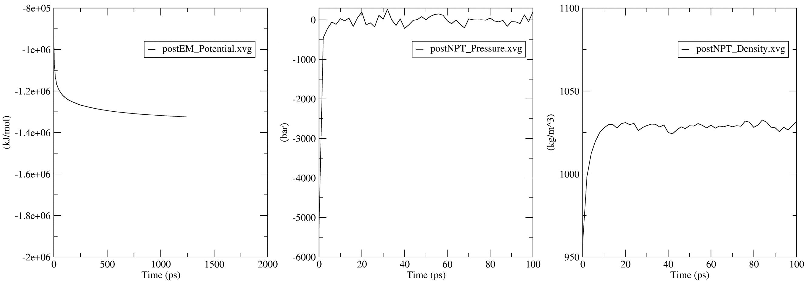
The values above have been arrived at by adjusting the coordinates such that it is wide enough to contain the complex even after the pulling simulation whilst taking care of the periodic boundary condition. At the next prompt, choose to proceed with the next steps, and CHAPERONg would execute the solvate, add ions, and the energy minimization steps. Thereafter, you would be prompted to indicate if you need to make a special index group. Enter “no” and CHAPERONg would take care of the index groups for you automatically. For most users, this would be sufficient, but if you need to make some other index groups, then feel free to do so. Next, you would need to indicate at the next prompt whether you would like to carry out an optional NVT equilibration. This is generally not necessary and you can enter “no”, but if you wish to run it, make sure to have a suitable nvt.mdp file in the working directory.

7. Steered MD Simulation

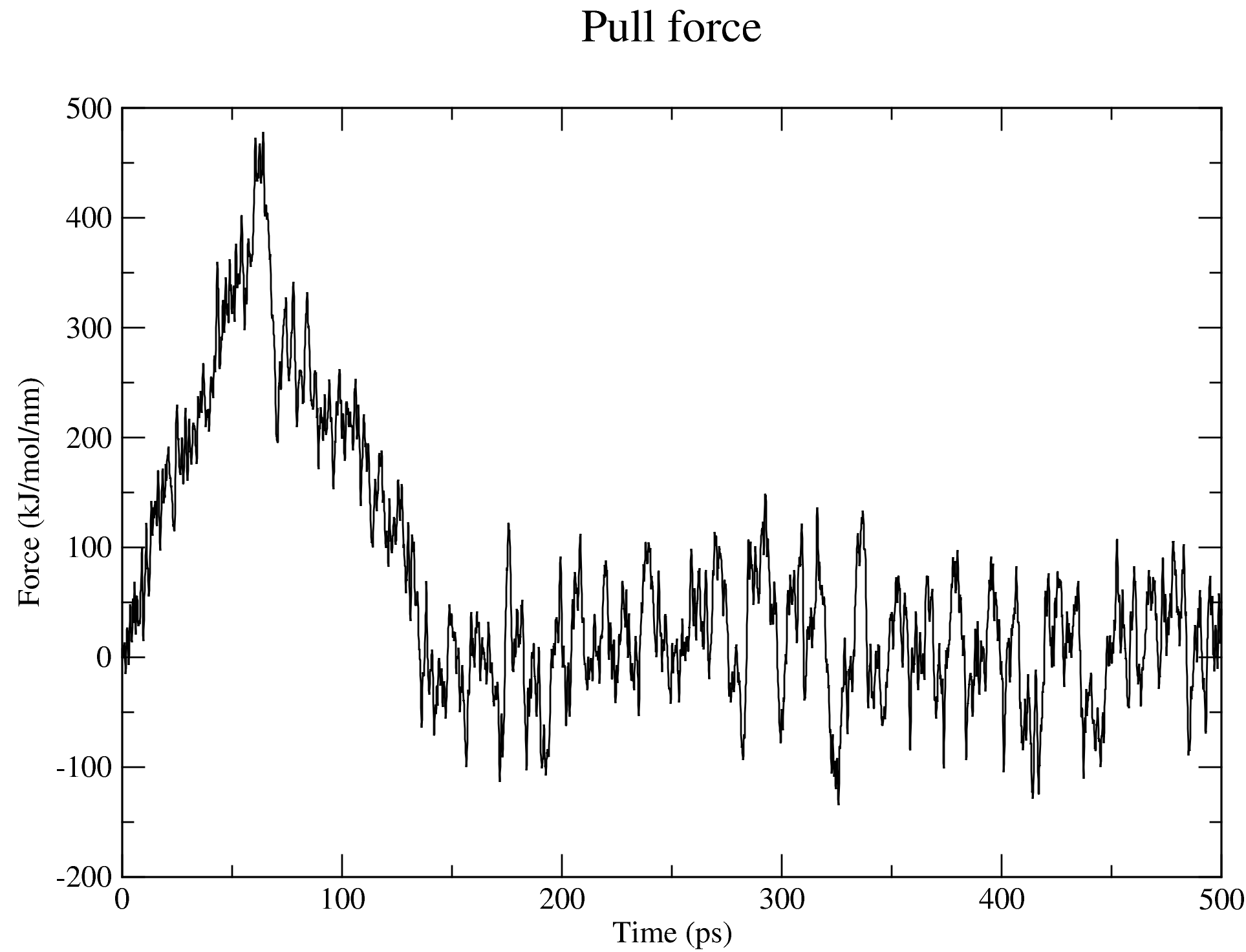
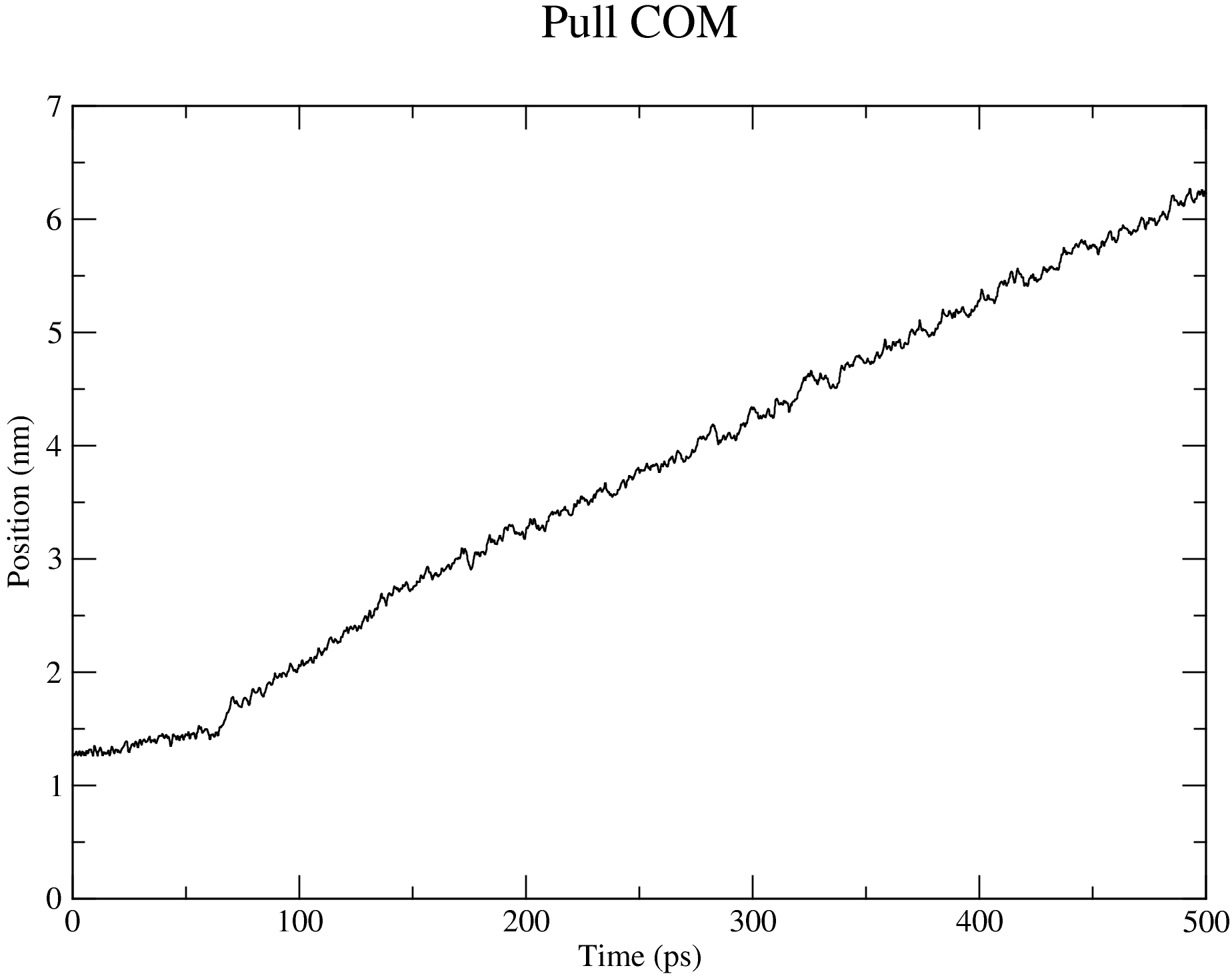
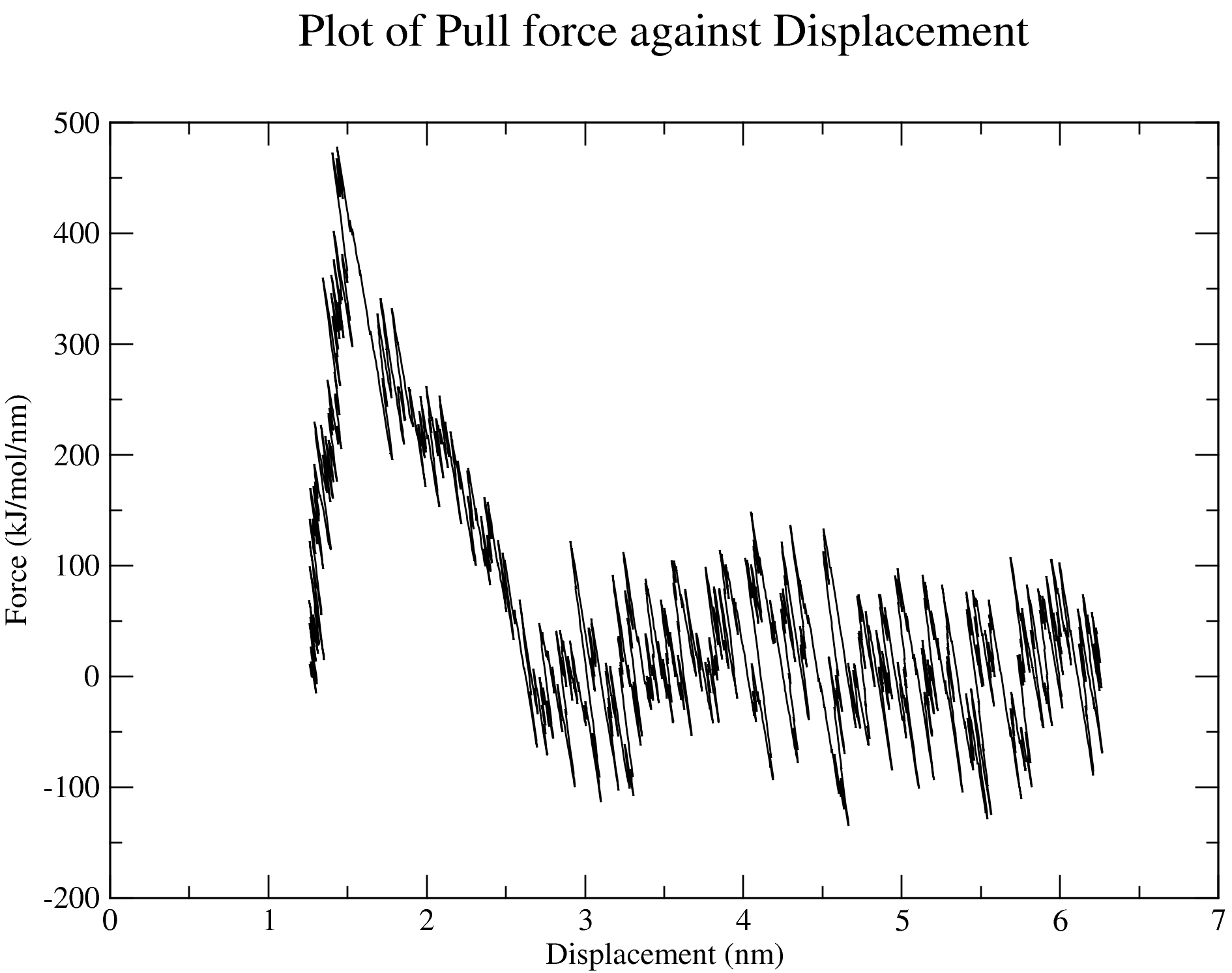
The nsteps, dt, and the pull_coord1_rate parameters set in the md_pull.mdp file contained in the folder that you have downloaded indicate that we will be pulling the ligand away from the receptor for 500 ps over a distance of 5 nm in the z-direction. And this pulling will take place in a box of size 14 nm in the direction of the pulling as specified in the box definition discussed above. You can adjust these parameters based on your specific case. The output files of the pulling simulation, including the ones shown in the figures below, are saved in the folder steered_MD.

8. Movie of the Steered MD Simulation

Immediately after the steered MD simulation, a movie of the simulation is made after which the subsequent steps would follow. You can use the protocol described in the previous Tutorials to adjust the movie as you desire.

9. Umbrella Sampling, PMF and WHAM

Based on the 0.2 nm window spacing that we set (using the us_window_spacing in the paraFile.par file), 30 initial configurations were identified by CHAPERONg (see the configuratns_list.txt file). In the md_umbrella.mdp file, we set the nsteps parameter to 1000000 so that a regular MD simulation of 2 ns is sequentially run for each window to make a total of 60 ns for all the windows. Once umbrella sampling is completed for all the windows, the WHAM analysis is run to reconstruct the PMF curve. The figures below show the histograms of the umbrella windows and the PMF curve.

The calculted free energy of binding ${\Delta}G$ is written to the file summary_dG.dat. For the complex in this tutorial, the estimated binding energy is -11.855 kCal mol^-1. This value is not too far from the experimental binding energy of -9.36 kCal mol^-1 estimated from the reported ${K_i}$ of the complex using the expression below:

$$ {\Delta}G_{EXP} = RT{\ln}K_i $$

where,

• ${\Delta}G_{EXP}$ is the experimental free energy of binding (in kcal mol^-1) of the protein-inbitor complex,
• $R$ is the gas constant (in kcal mol^-1 K^-1),
• $T$ is temperature (in K), and
• $K_i$ is the experimentally determined inhibition constant.

I try my best to make the information on this website as accurate as possible, but if you find any errors in the contents of this page or any other page on this website, kindly get in touch with me at contact@abeebyekeen.com. Also, you are welcome to reach out for assistance and collaboration.