Tutorial 3: Automated MD Simulation of KEAP1 Kelch Domain-Inhibitor Complex

A tutorial on how to use CHAPERONg for automated GROMACS MD simulation of a protein-ligand complex & post-simulation analyses.
0. Introduction
This is the third in the CHAPERONg tutorial series. In this tutorial, I assume that the reader is familiar with CHAPERONg or has already gone through the preceding Tutorials 1 and 2. Some of the basics covered in those tutorials will not be repeated here; only the aspects and tips that are unique to the GROMACS MD simulation of protein-ligand complexes will be focus on. In particular, this tutorial will be a follow up to Tutorial 2 where we carried out the MD simulation of the Kelch domain of the human KEAP1 apoprotein (KEAP1kd). In the PDB structure that we used in that tutorial, the protein was stripped of all ligand coordinates. Here, the same PDB structure will be used, but we will keep and use the coordinates of the small molecule inhibitor co-crystallized with the protein. The KEAP1kd and the inhibitor will be simulated as a complex in water. Then, we will carry out some trajectory analyses, especially those that relate to binding events.
- Fully automated run of a 100 ns MD simulation of the KEAP1kd-inhibitor complex in water using the
fullautomation mode of CHAPERONg. - Automatic selected post-simulation analyses of the trajectory:
1. Preparing the Starting Structure
The starting structure for this simulation will be the same as the one we used in Tutorial 2 (i.e. the human KEAP1 Kelch domain in complex with a small molecule inhibitor—PDB ID 4IQK). Download the coordinates file from the RCSB PDB and copy it into the working directory where you will be running the simulation.
Crystal structures are often not without deficiencies. These include problems such as refinement inadequacies, as well as missing atoms and residues that could not be placed in the electron density. For researchers with the appropriate expertise, it is always a good and encouraged idea to inspect the electron density map of the structure of interest to ensure that the PDB model fits the density well enough, especially at regions of particular importance to the study. Fortunately, the 4IQK structure which we will be using in this tutorial is free from any major defects and can be directly used for MD simulation. If the structure you would like to use has missing atoms or residues, or has some other problems, click here to see the guide provided in Tutorial 1.
2. Cleaning up the Starting Structure
We are going to remove all the ligands in the crystal structure and then save the protein and the small molecule ligand of interest (the inhibitor co-crystallized with the protein) as separate PDB files. This may not always be the best practice in all cases. However, for the purpose of this tutorial, we are not interested in other moieties aside from the two. Enter the command below to extract the apoprotein and save it as KEAP1kd.pdb.
|
|
Then, extract the inhibitor and save it as IQK.pdb :
|
|
Then, add hydrogen atoms to the IQK ligand and save/convert it to a .mol2 file. To do these with PyMOL, open the ligand in PyMOL while in the working directory:
|
|
Run the following set of commands, one line after the other (and, of course, excluding the “PyMOL>” string), on the PyMOL command line:
|
|
You can also achieve all of the cleaning steps above using any of your favorite visualizers (PyMOL, Chimera, Discovery Studio, Maestro, etc.). To follow along in this tutorial, you may download a copy of each of the cleaned protein and ligand here and here, respectively. To download the all-atom IQK.mol2 from the step above, click here.
Note that we have added all H atoms to the IQK ligands since the force field we are using in this tutorial is the CHARMM—which is an all-atom ff. Be aware that if you need to assign computed protonation state for the ligand (or protein) in your case, you might be better off using other tools/servers that compute pK values of ionizable groups in macromolecules. There are many options to choose from, including the H++, Epik (in Maestro), PROPKA, MCCE, PlayMolecule-ProteinPrepare, etc.
3. Forcefield Files
GROMACS automatically supports a number of forcefields, many of which are provided by default upon GROMACS installations. The list and details of the supported forcefields, including AMBER, CHARMM, GROMOS, and OPLS, and their various distributions are provided in the relevant part of the GROMACS documentation. You can select and use the one that best suits your purpose. In this tutorial, we will be using the CHARMM36 forcefield, the latest version of which you can download from MacKerell Lab website. From the same web page, you should also download the cgenff_charmm2gmx_py*_nx*.py python script appropriate for the python version on your machine. Copy the downloaded charmm36-***2022.ff.tgz and cgenff_charmm2gmx_py*_nx*.py files into the working diectory and run the command below to unpack the forcefield:
|
|
4. Ligand Topology
To generate the ligand topology information for the CHARMM3 forcefield, go to the CGenFF (CHARMM General Force Field) webserver and create an (/login to your) account. Upload IQK.mol2, wait for the output .str CHARMM-compatible “stream file” to be produced. Click on the IQK.str link and it will open in another tab of your browser. Copy the content of the page, open your favourite text editor, paste it in and save the file as IQK.str into the working directory. The CGenFF webserver provides penalty scores associated with the parameterized ligand which you will find in the content of IQK.str. According to the usage guide of the CGenFF webserver, penalties scores lower than 10 indicate that the parameterization can be considered to be reliable for use directly, scores between 10 and 50 imply that some basic validation is recommended, and scores above 50 indicate that additional optimization are required. For the IQK ligand in this tutorial, you will find that all the penalty scores are (unusually) zero, indicating that the parameterization is very reliable. You can have a look at a copy of the generated IQR.str file here.
5. GROMACS and CHAPERONg Parameters
Next, you will edit the paraFile.par file to set the CHAPERONg parameters for the simulation. You also need to provide the GROMACS MD simulation parameters (mdp) files. Copy the mdp files into the working directory and name them as follows:
- ions.mdp – mdp for the adding ions step
- em.mdp (or minim.mdp) – mdp for the energy minimization step
- npt.mdp – mdp for the NPT equilibration step
- nvt.mdp – mdp for the NVT equilibration step
- md.mdp – mdp for the production simulation step
To follow along in this tutorial, you can click here to download a folder containing all the input files for the simulation, including the prepared protein, ligand, paraFile.par, mdp, topology and forcefield files. Extract the folder and cd into it:
|
|
|
|
6. Launching CHAPERONg
The nsteps parameter in the md.mdp file is set to 50000000 so the simulation would run for 100 ns. You may reduce this value to a number that the computing power of your device can conveniently handle. Open paraFile.par with a text editor to see what parameters have been set for the run. The command below launches CHAPERONg with the parameters in paraFile.par parsed to it.
|
|
Alternatively, you could also launch CHAPERONg using one of the more verbose commands below:
|
|
|
|
Proceed with the simulation by selecting “protein-ligand complex” as the type of syste being simulated and starting from the very first stage “0a”. Enter “IQK” as the name of the ligand. After the protein topology is generated, you will be prompted to select the platform/forcefield through/with which your ligand topology has been derived. For this tutorial, we generated the topology parameters for the IQK ligand using the CHARMM general forcefield (CGenFF) server, and we will proceed accordingly.
CHAPERONg also automates GROMACS MD simulation for complexes whose ligand topologies have been generated with the ACPYPE (for AMBER), the LigParGen (for OPLS), or the PROGRG2 (for GROMOS) tools/webservers. Upload the ligand molecule to the server of interest and download the generated topology files as a compressed file. Extract the compressed file and rename the folder/subfolder containing the ligand topology as ligpargen, acpype, or prodrg, as the case may be. Then, simply place the renamed folder into the working directory before launching CHAPERONg.
The simulation would proceed till the completion of the production run, and multiple output data would be generated as shown in the preceding tutorials. Check the quality assurance analyses data to monitor your simulation and ensure that things go well.
7. Post-simulation Trajectory Analyses
Once the production run is completed, you will be prompted to choose whether to proceed with post-simulation trajectory analyses. Enter yes to do so. From the list of analyses presented to you, enter 21 to run all the analyses save “Clustering” and “g_mmpbsa”. These would typically be run later after some other analyses have been completed and some insight obtained about the trajectory. In this tutorial, we will only look at the result of some the analyses. For details of other analyses that aren’t covered in this tutorial as well as more information about some of those covered, see Tutorials 1 and 2.
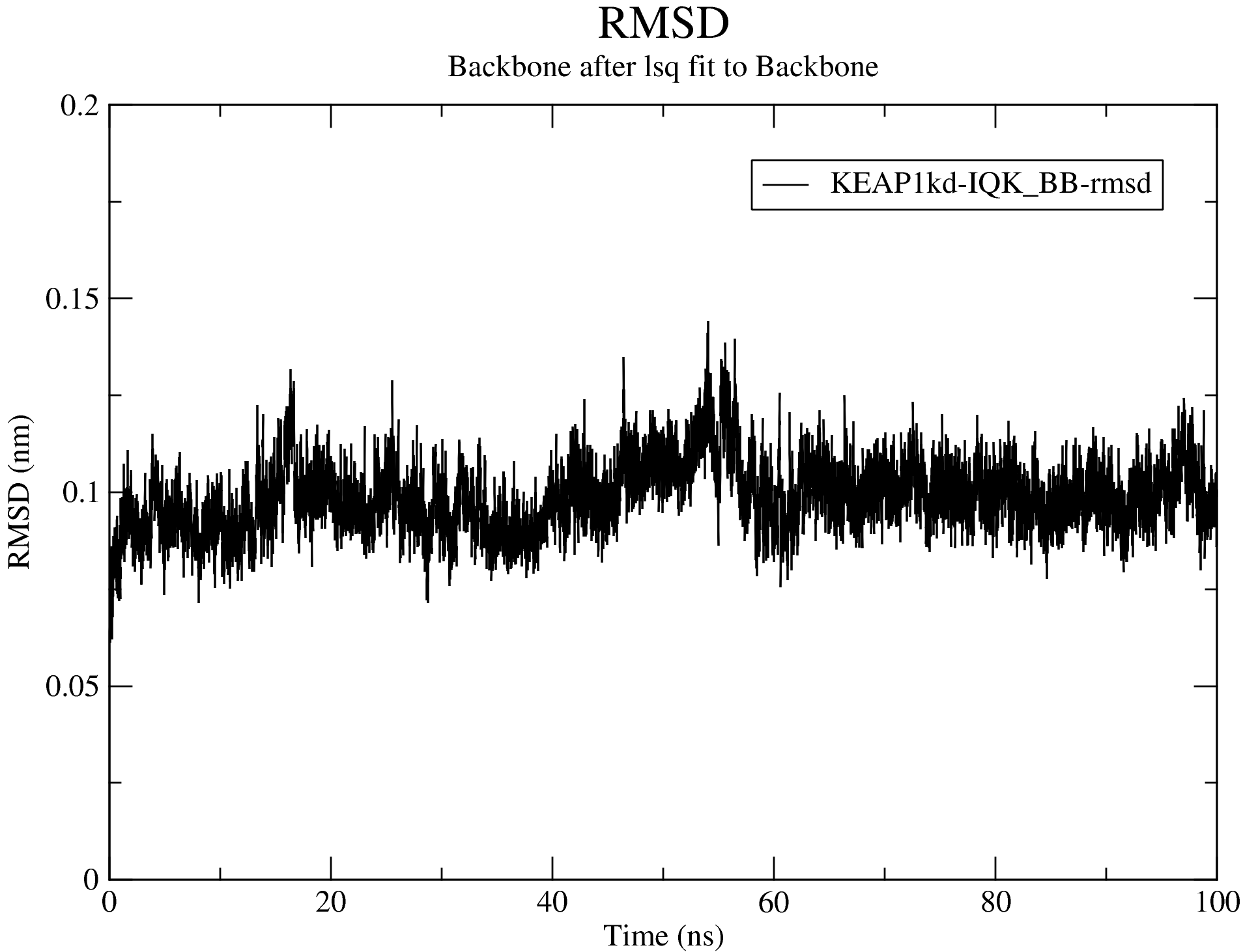
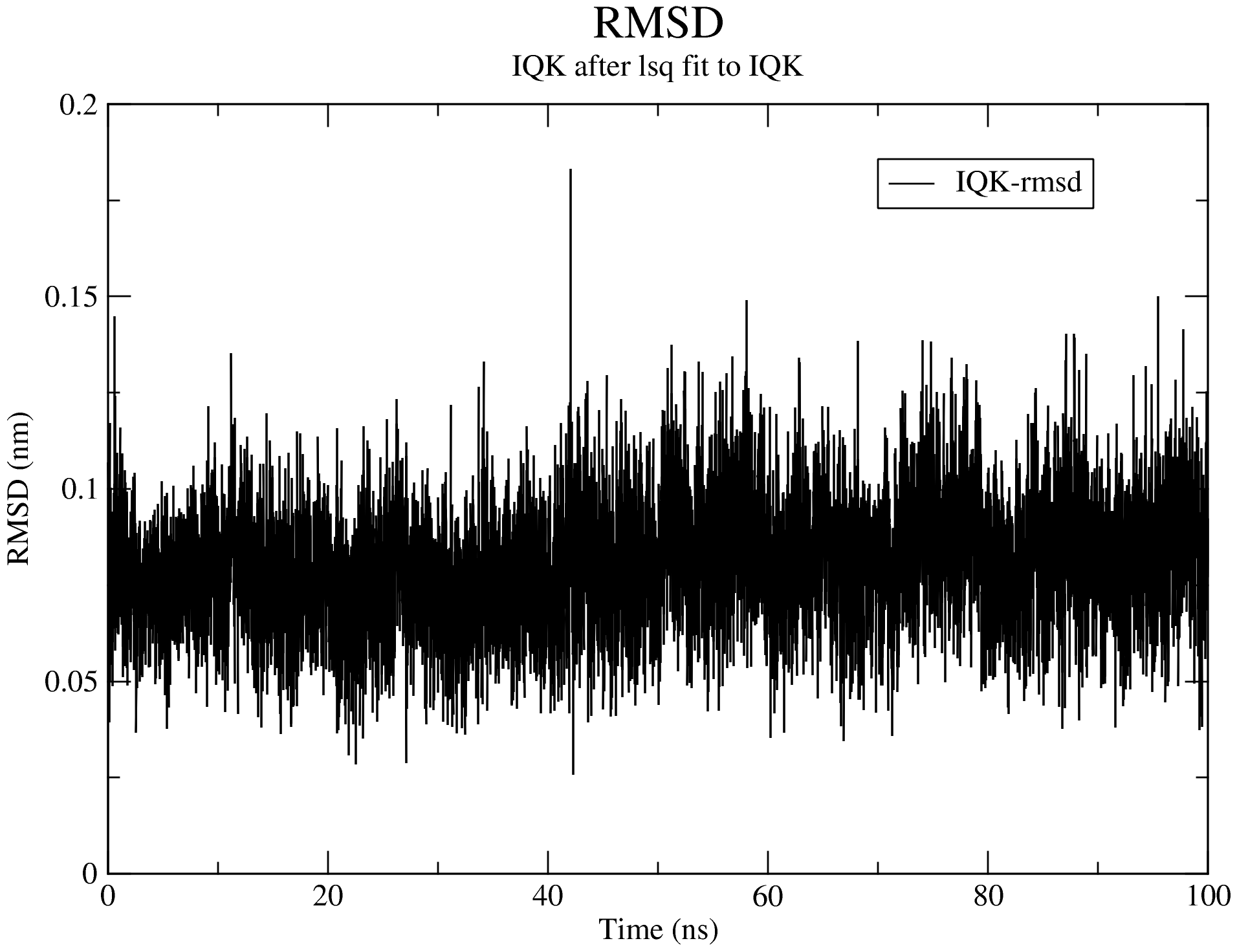
7.1. Root Mean Square Deviation (RMSD)
For details of the output produced for the RMSD calculations, see the RMSD section of the documentation.
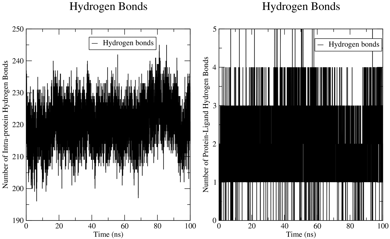
7.2. Hydrogen Bonding Analysis
Being a protein-ligand system, the hbond calculations passed to GROMACS by CHAPERONg include the numbers of protein-solvent hbonds, intramolecular (intra-protein) hbonds, and protein-ligand hbonds. For more details, see the hydrogen bond analysis section of the documentation.
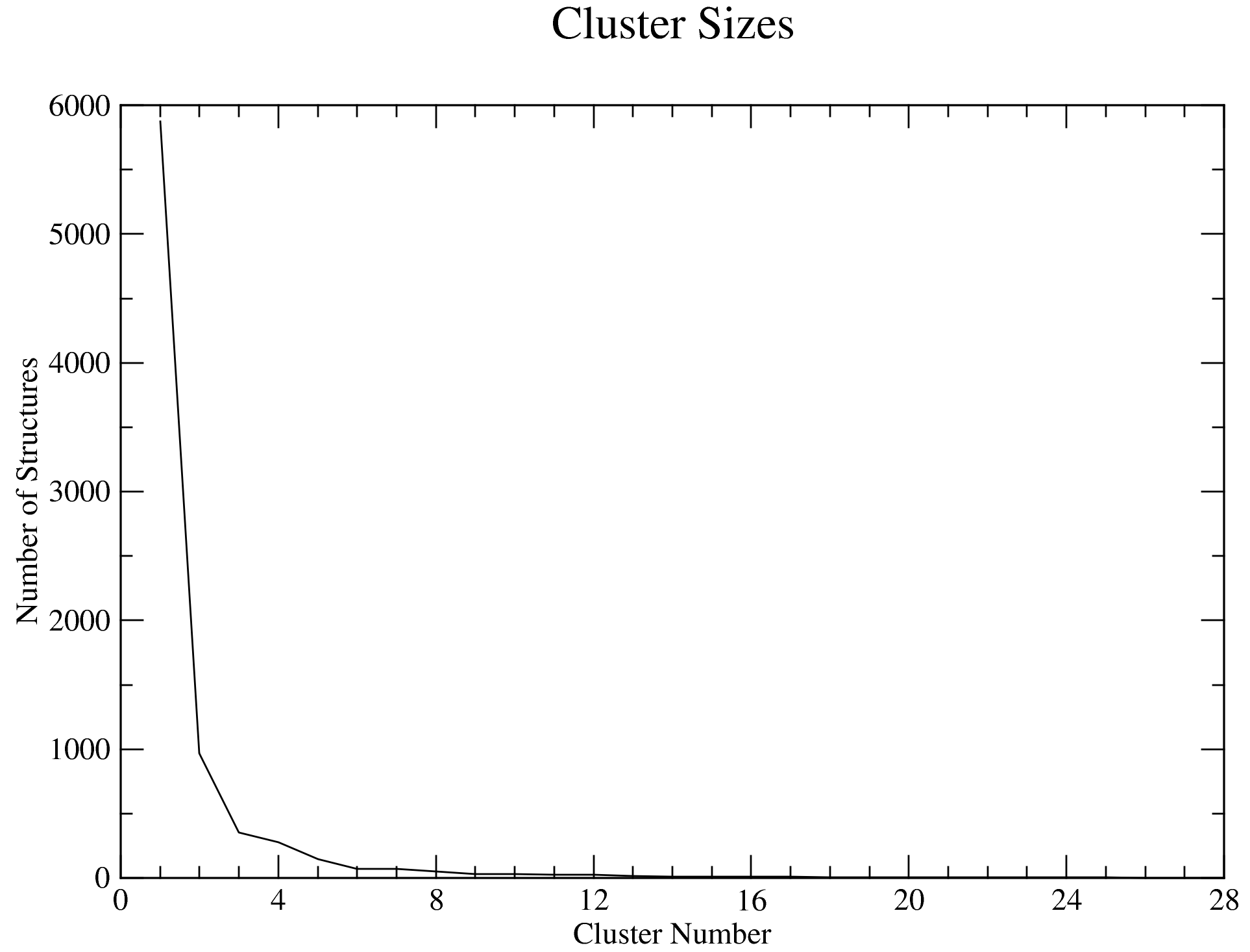
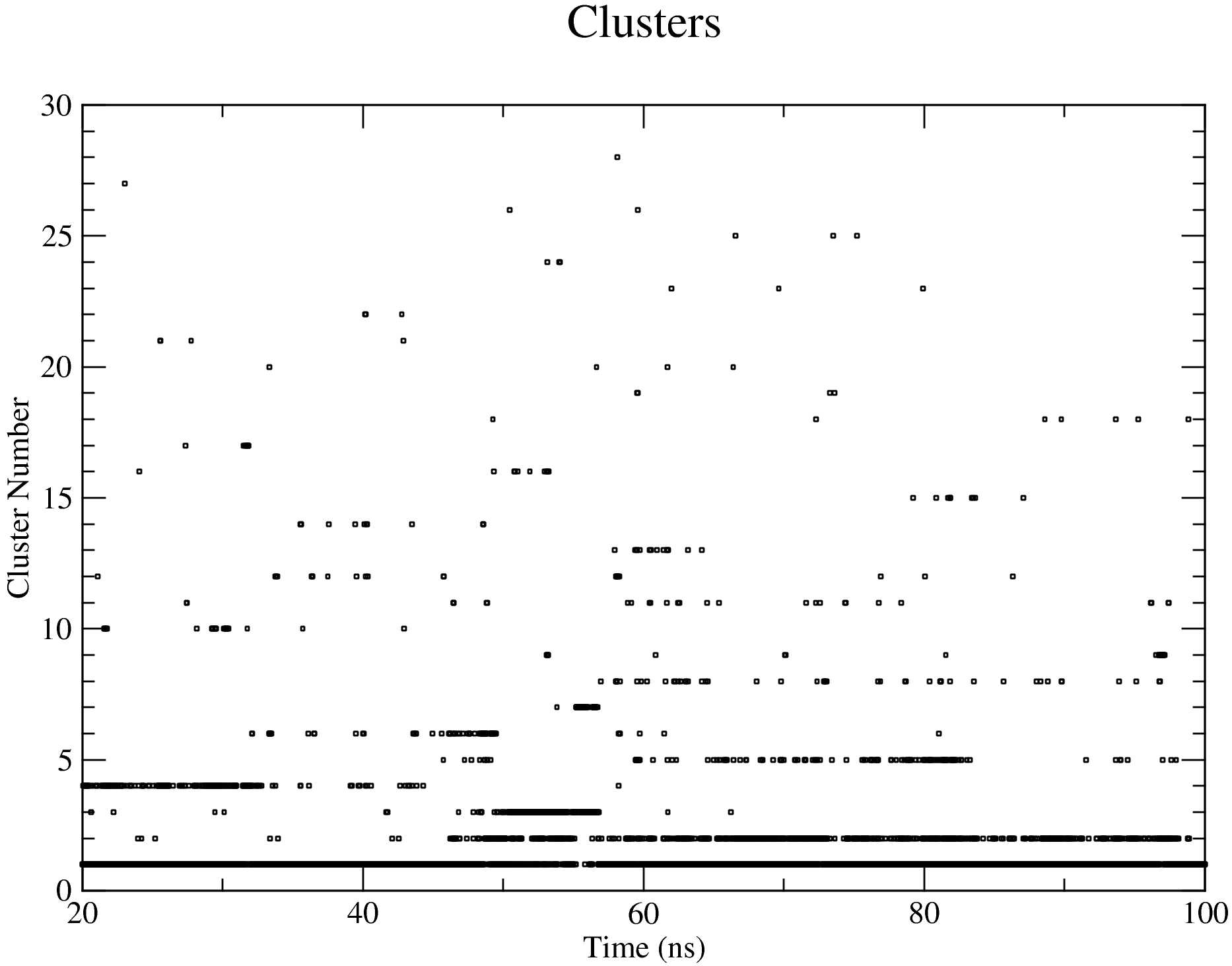
7.3. Clustering Analysis
Looking at the data from the completed analyses, we now have an idea of what the trajectory is like. For example, the RMSD plot above shows that complex is very stable all through the simulation duration, with the backbone RMSD hovering around 1 Å. We also see that the system reached equilibrium before 20 ns. Thus, we will set the frame_beginT parameter in paraFile.par to 20000 (ps) to consider all frames recorded after the 20 ns timestamp. Using the gromos clustering method (Daura et al.1999), the RMSD cut-off for two structures to be considered as neighbours will be set to 0.08 (using the paraFile.par parameters clustr_methd and clustr_cut, respectively). This cut-off was chosen as the optimal value after multiple trials, and it is this small because of the high stability of the system. You can update these parameters in your paraFile.par, or click here download a copy of the updated CHAPERONg parameter file (now named paraFile_updated1.par simply to differentiate it from the first one). Have a look at the parameter file and compare it with the previous one to see the differences. For more details of all the available options, see the clustering section of the documentation. To launch CHAPERONg for the clustering analysis, run the following command:
|
|
Or this (if you modified the previous parameter file):
|
|
We could also choose to simply add the new parameters to the command without editing paraFile.par:
|
|
The output files will be saved into the Clustering folder. The log file shows that, with the set cut-off, 28 clusters were identified and the representative structures for all the clusters are saved as clusters_representatives.pdb. Figures of some of the clustering details, including the cluster sizes and the distribution of the cluster members across the simulation time, are shown below:
7.4. Simulation Movie
The paraFile.par parameter movieFrame was set to 250 so that 250 frames are taken across the trajectory to generate a movie. For more details about simulation movie, see the relevant section of the documentation.
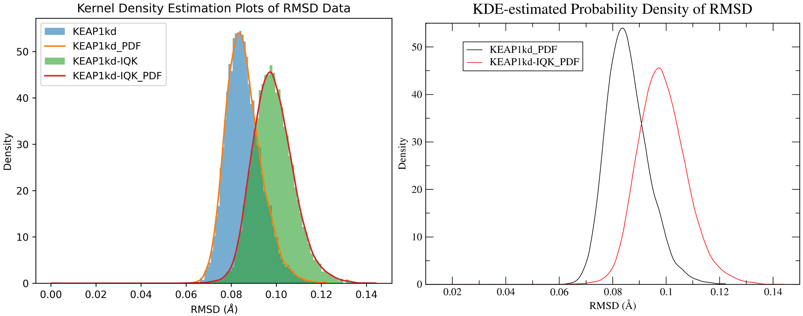
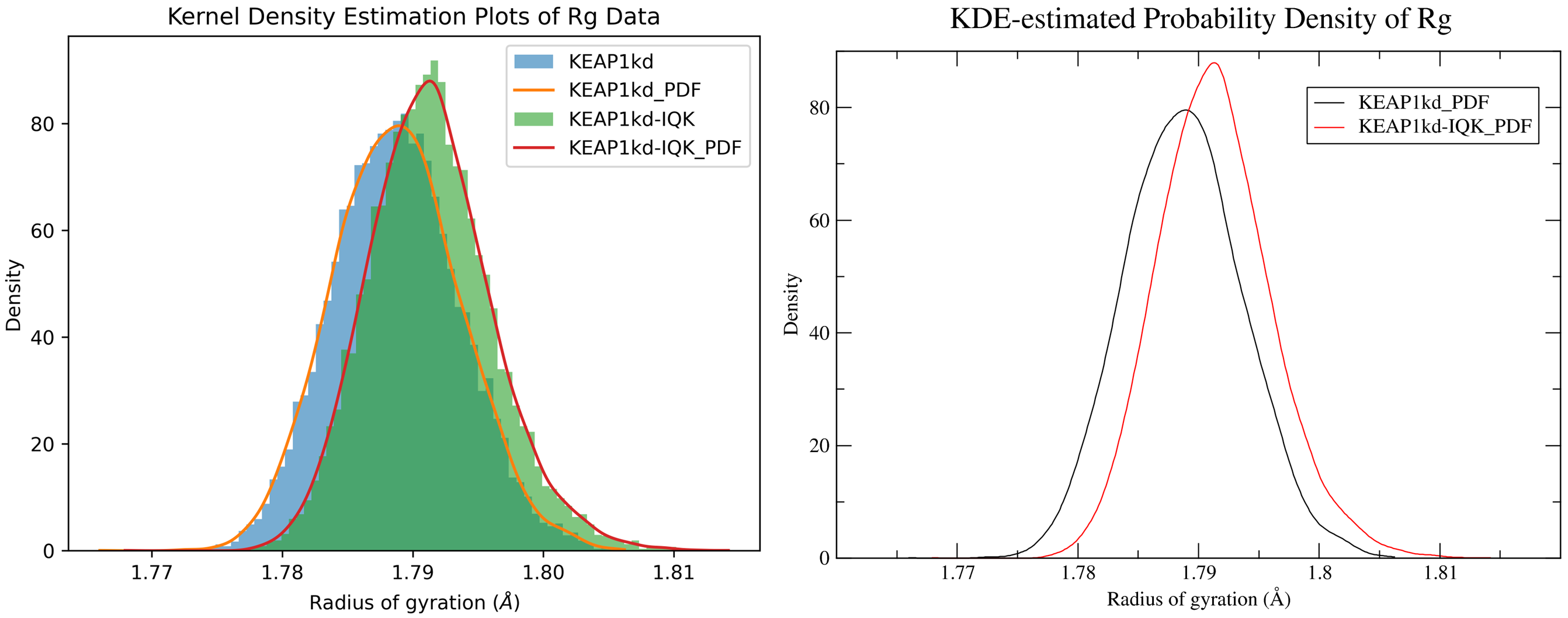
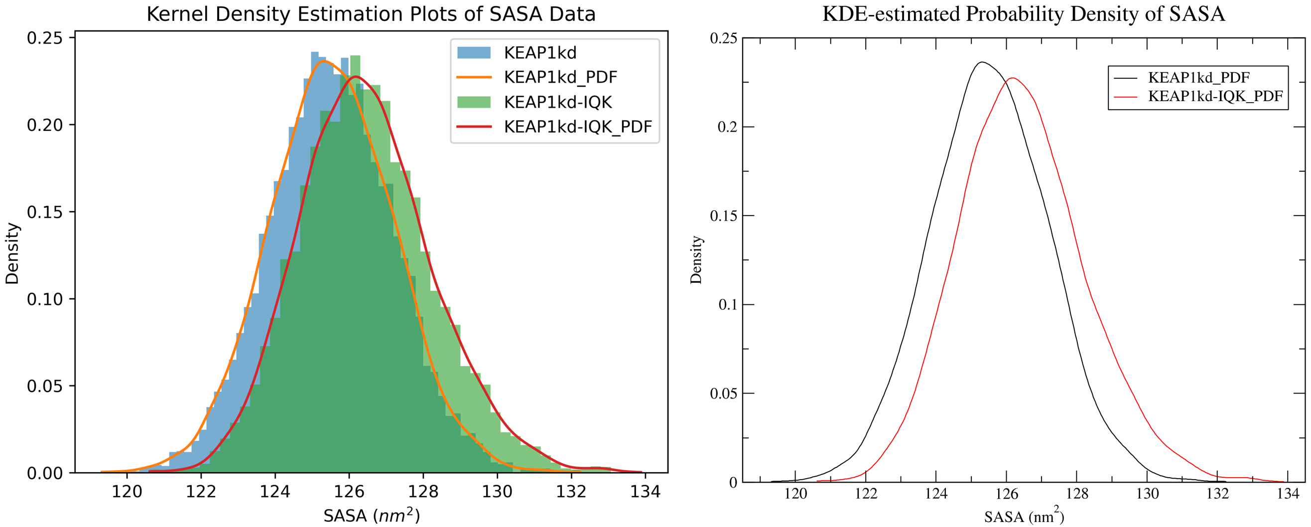
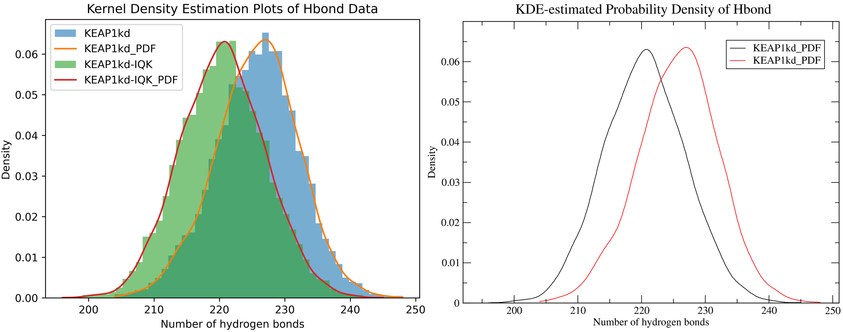
7.5. Kernel Density Estimation for Comparing Multiple Datasets
By running CHAPERONg in the full auto mode and using the --kde_opt parameter (see the relevant section of the documentation for more details), identify the optimal number of bins for plotting KDE for RMSD, Rg, hbond and SASA (see Tutorial 2). Using the optimal number of bins, we will now generate multi-data KDE plots to compare the data from the current KEAP1kd-IQK complex MD simulation with those of the previous KEAP1kd apoprotein MD simulation run (in Tutorial 2). Below are the multi-data KDE plots of the RMSD, Rg, hbond and SASA data. The figures generated from the .XVG output of CHAPERONg for each plot are also shown.
7.6. g_MMPBSA Free Energy Calculations
To launch CHAPERONg again—this time for g_mmpbsa calculations—run the command below, noting that g_mmpbsa-related parameters have been set in paraFile.par.
|
|
Alternatively, you could also launch CHAPERONg using one of the more verbose commands below, in which case the g_mmpbsa-related parameters are provided on the command line:
|
|
For detailed information about the parameters provided for the g_mmpbsa run above, see the relevant section of the documentation. After the g_mmpbsa run above, the output files, including those containing the estimated breakdown of the energies, total binding energy, residue-wise energy contributions, etc., are saved in the folder MMPBSA in the working directory.
Related: BioMoDes: Conformational Ensemble & Dynamics Analysis Tools | CHAPERONg Documentation
I try my best to make the information on this website as accurate as possible, but if you find any errors in the contents of this page or any other page on this website, kindly get in touch with me at contact@abeebyekeen.com. Also, you are welcome to reach out for assistance and collaboration.