Automated MD Simulation Trajectory Analyses - Part II

CHAPERONg introduces the estimation of PDF using the KDE for further analysis of several analysis data that are often generated from MD simulation trajectory. This would help to not only visualize and understand the distribution of the data, but also to calculate statistics of interest. KDE estimation in CHAPERONg is carried out using the the SciPy python package, which implements the Gaussian kernel.

Given a sample $ x = {x_{1}, x_{2},…, x_{n}} $ with an unknown density $ f $ at any given point $ x $. The kernel density estimator of the shape of this function $ f $ is defined as expressed in equation (1) below:

where,

• $ K $ is the kernel (a simple non-negative function such as the Gaussian distribution), and
• $ h > 0 $ is the smoothing bandwidth (a real positive number that defines smoothness of the KDE plot).

As shown in the image below, the KDE probablity density function estimation in CHAPERONg can be carried out on a single dataset to plot a curve, or to plot a combined set of curves for multiple datasets of the same type (often for the purpose of comparison).

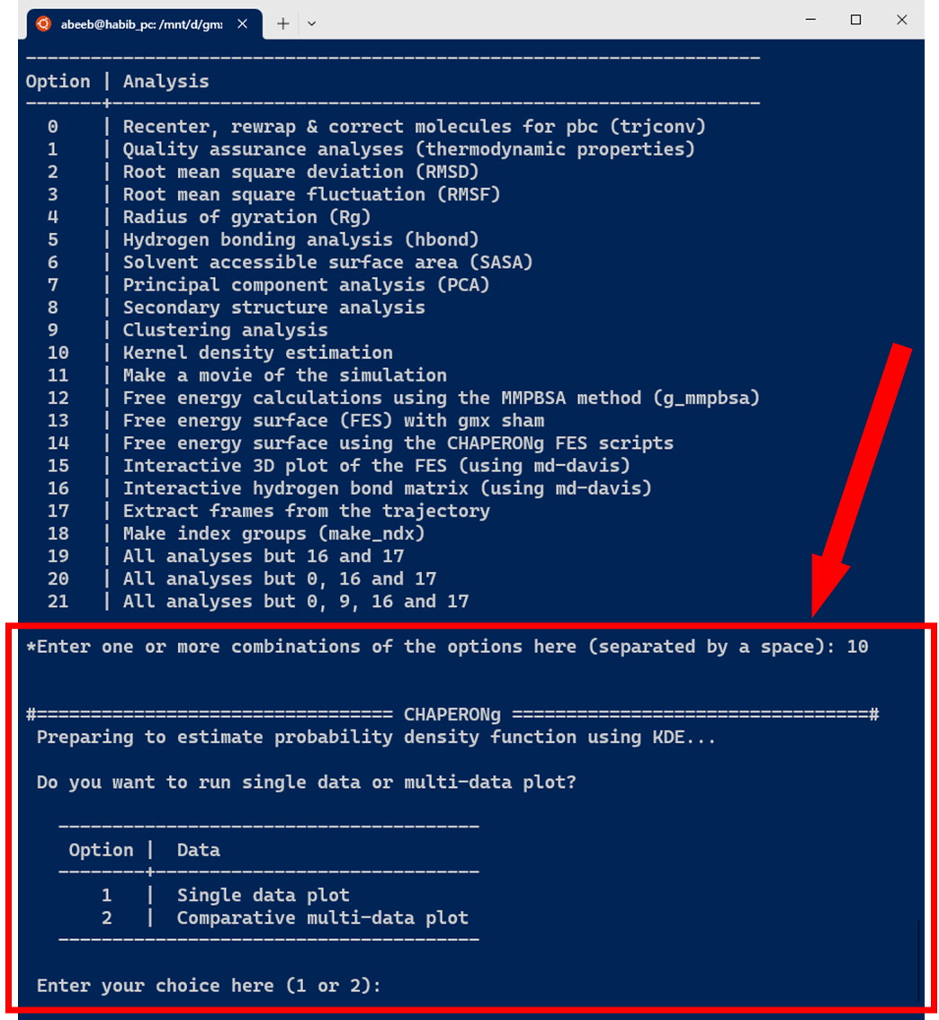
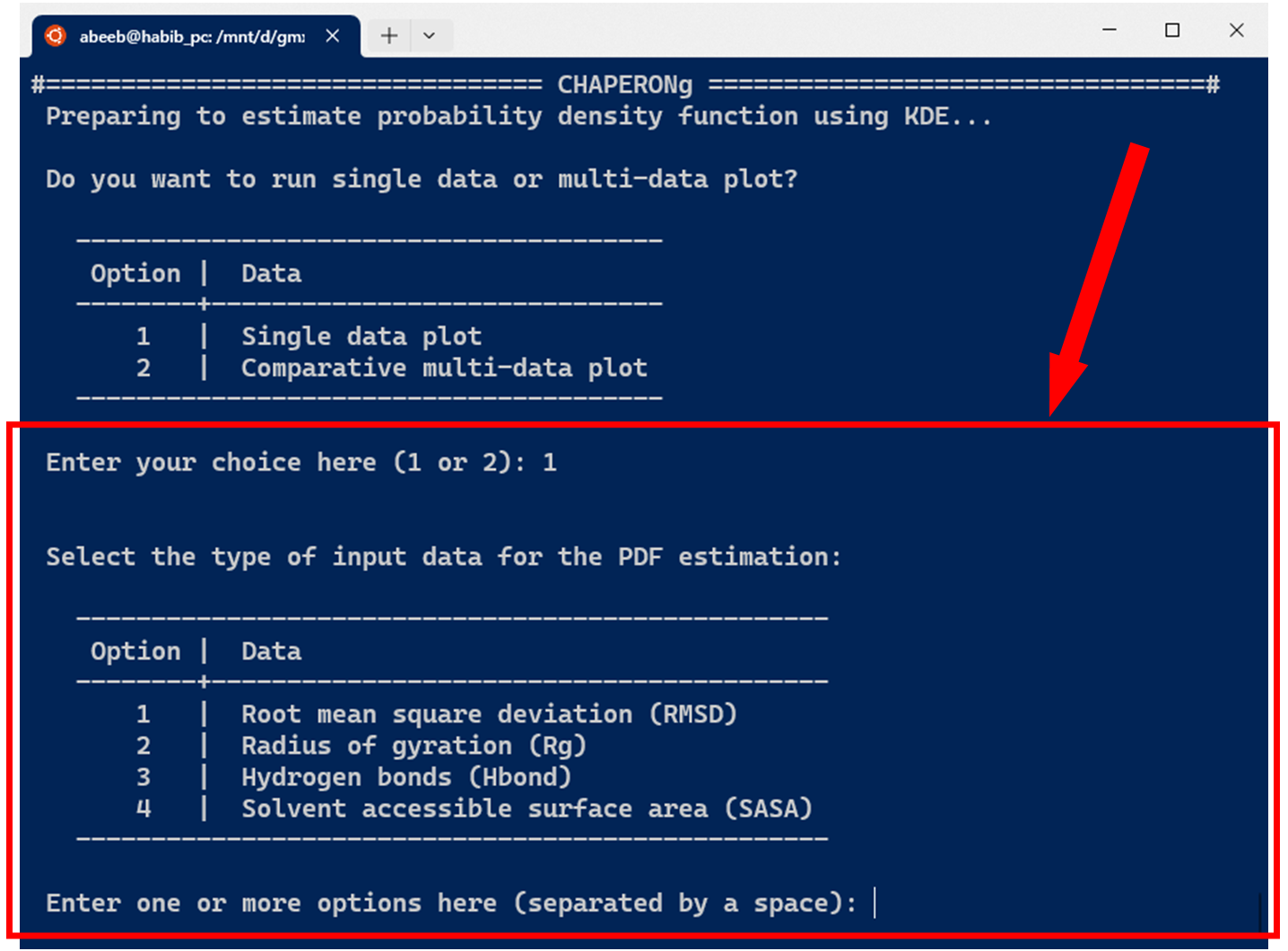
The current version of CHAPERONg supports the estimation of PDF for four types of data commonly obtained from MD simulation, including the root mean square deviation (RMSD), radius of gyration (Rg), hydrogen bonds (Hbond), and solvent accessible surface area (SASA). As shown in the image below, one or more input data can be specified.

10.1. KDE plot for single datasets

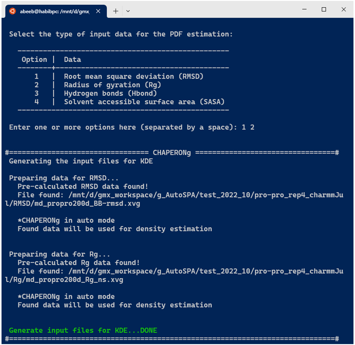
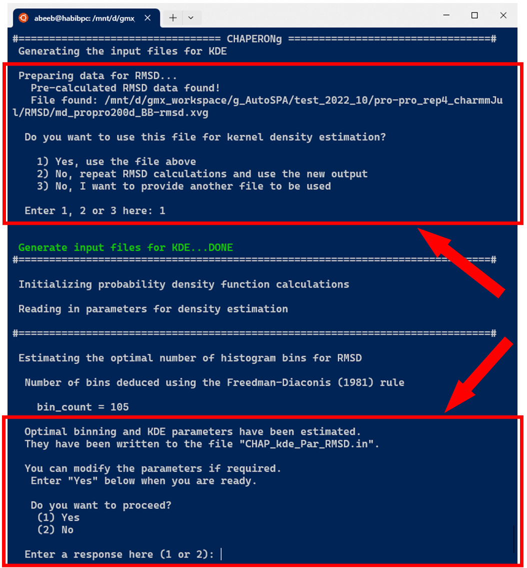
In the case of running KDE for single data plots, an example run for RMSD KDE is shown below. After selecting the choice of input data from the options, CHAPERONg checks the working directory for the existence of a pre-calculated input data. If there exists one, this is used as the input for the PDF estimation (as is the case in the example run shown in the image below). Otherwise, the RMSD, Rg, Hbond, or SASA analysis is first executed and the output is parsed to the CHAP_generate_kde.py script for the PDF estimation.

A subfolder named Kernel_Density_Estimation is created (in the working directory) by the code. If such a directory from a previous KDE run exists, it is backed up by renaming it before the new folder for the current run is made. The optimal number of bins to be used in the generating a 2D histogram of (each of) the data is estimated using multiple estimators. These include the Freedman-Diaconis (1981), the Scott(1979), the Rice (1944), and the square-root methods, expressed in equations 2, 3, 4, and 5 below, respectively.

$$ \tag {2} Number_{bins} = ceil\left(\vcenter{\hbox{$\dfrac{max(data) - min(data)}{2 \cdot \cfrac{(q_{3} - q_{1})}{\sqrt[3]{n}}}$}}\right) $$

$$ \tag {3} Number_{bins} = ceil\left(\vcenter{\hbox{$\dfrac{max(data) - min(data)}{3.5 \cdot \cfrac{\sigma}{\sqrt[3]{n}}}$}}\right) $$

$$ \tag {4} Number_{bins} = ceil \Big( 2 \cdot {\sqrt[3]{n}} \Big) $$

$$ \tag {5} Number_{bins} = ceil \Big( \sqrt{n} \Big) $$

where,

The estimated number of bins for each method is written to the files kde_bins_estimated_summary.dat and kde_bins_estimated_$<$input-data$>$.dat (or a series of such files in the case of several input data).

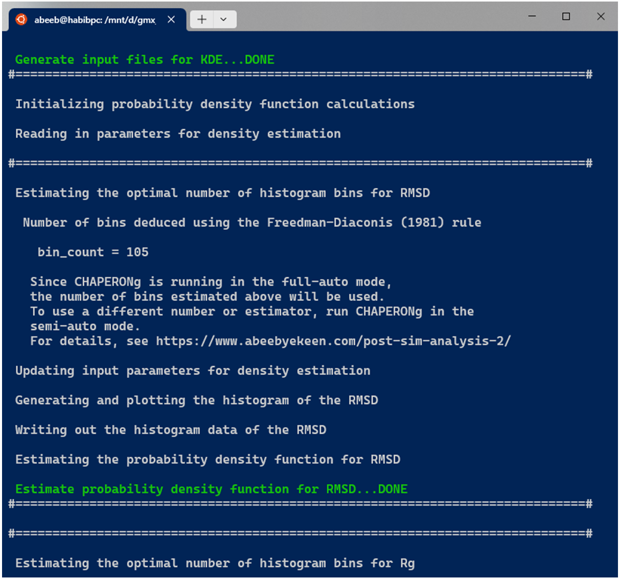
When CHAPERONg is run in the full-auto mode, the number of bins estimate deduced from the Freedman-Diaconis (FD) rule—because it is robust and takes into account data variability and size—is automatically used for generating the 2D histogram. This is the case with the example run shown in the snapshot above. To have more control over the choice of the estimator or to use a custom number of bins, CHAPERONg can be run in the semi-auto mode where the user is prompted to confirm whether to use the automatically calculated FD estimate of the number of bins. At this point, the input parameter file CHAP_kde_Par_$<$input-data$>$.in can be modified to change the number of bins specified by the bin_count parameter. In addition, the smoothing bandwidth $h$ of the KDE can be set by modifying the bandwidth_method parameter in the same input parameter.

The bandwidth determines the width of the kernel, and it represents an important parameter when calculating the KDE. The larger the bandwidth value, the smoother the estimate gets, tending towards oversmoothing; and the smaller bandwidth, the more jagged the estimate, tending towards undersmoothing. The SciPy package supports automatic bandwidth selectors including the Scott’s (1992) and Silverman’s (1986) rules-of-thumb defined in equations (6) and (7), respectively, as well as custom bandwidth values (float). The Scott’s and Silverman’s rules are implemented in Scipy’s gaussian_kde as scotts_factor and silverman_factor, defined in equations (8) and (9) below, respectively. The Silverman’s rule is set as the default in CHAPERONg because it is widely used and is often considered a reasonable default choice.

$$ \tag {6} h = \left( \frac{4\hat{\sigma}^5}{3n} \right)^{\frac{1}{5}} \approx 1.06\cdot\hat{\sigma}n^{{-1}/{5}} $$

$$ \tag {7} h = 0.9\cdot min \left( \hat{\sigma} , \frac{IQR}{1.34} \right) n^{{-1}/{5}} $$

$$ \tag {8} scotts\text{\textunderscore}factor = \left( \frac{1}{n} \right)^{\frac{1}{d + 4}} $$

$$ \tag {9} silverman\text{\textunderscore}factor = \left( \frac{4}{n\cdot(d + 2)} \right)^{\frac{1}{d + 4}} $$

where,

• $ h $ is the bandwidth,
• $ \hat{\sigma} $ is the standard deviation of the dataset used to scale the bandwidth,
• $ IQR $ is the interquartile range (i.e. Q3 - Q1),
• $ n $ is the size of the dataset,
• $ d $ is the number of dimensions.

The output files generated by CHAPERONg include the .PNG and .XVG files of the histograms and KDE plots. In addition, a file listing the statistics (the mean, the standard deviation, the minimum and the maximum data points, and the mode(s)—i.e. the most frequent values) of each data set is generated and saved in the Kernel_Density_Estimation folder.

For some data, it might be challenging to employ the trial-and-error (sort of) approach described above to identify the optimal/best number of bins to use for the 2D histogram. CHAPERONg offers a way to automatically test a range of number of bins around the FD estimate in a systematic fashion. To use this approach, use the --kde_opt flag on the command line at the launch of CHAPERONg. This flag requires a number (integer) as parameter. CHAPERONg will generate a series of histograms using as number of bins values in the given range above and below the FD estimate (e.g. --kde_opt 30 will produce 60 histograms with 30 having the number of bins above the FD estimate, and 30 with number of bins below the estimate. Each histogram will have the corresponding number of bins as prefix to it’s figure name).

10.2. KDE plot for multiple comparable datasets

For combined multi-plot KDE, the user is prompted to provide the path to each of the data to be used for the PDF estimation. An example run for multiple RMSD data is shown in the snapshot below:

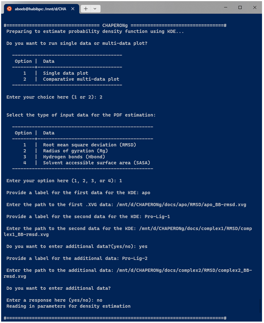
After providing the input data for KDE as shown above, all the subsequent steps are the same as those described earlier for the single plot KDE.

11. Free energy calculations using the MMPBSA method

11.1. Installing a compatible GMX or g_mmpbsa version

The g_mmpbsa package is a widely used tool for MM-PBSA calculations. It integrates with the GROMACS and the APBS packages for the calculation of binding energy and energy contributions of residues. However, the original g_mmpbsa does not work with recent versions of GROMACS without first re-processing the .tpr file from a GMX MD simulation. A common approach to doing this is to install a second copy but older version of gmx (version 5.x or lower). This is all you need to do and CHAPERONg will automatically handle the rest.

If you do not want to install the pretty old versions of GMX, you can try to instead compile a modified version of the original g_mmpbsa code that is supposed to provide supports for GMX version 2021 and older.

11.2. Providing the path to the GMX version to use

Once you have a g_mmpbsa-compatible GMX version installed, you need to provide CHAPERONg with the path to the gmx binary of this GMX installation for g_mmpbsa calculations. You could provide the path using the flag -M or --mmgpath on the terminal or via the paraFile.par file.

11.3. Input files and parameters to g_mmpbsa

Usually, you would use frames from a fraction of the trajectory, typically a certain last fraction of the simulation. To specify the fraction of the trajectory to use, CHAPERONg provides two options. One, you could specify the fraction of the trajectory to be used for the calculations using the --trFrac option (input is an integer; with 1 specifying the entire trajectory, 2 specifying the 2nd half, 3 for the last 3rd, 4 for the last 4th, etc.). Alternatively, you could use the --mmBegin parameter to indicate the time (in ps) to start reading the first frame from the trajectory. Further, you need to specify the number of frames to extract at intervals from the specified fraction using the --mmFrame option. When these parameters are not specified by the user, the default used by CHAPERONg are 100 frames extracted from the the last 3rd of the trajectory.

The precompiled g_mmpbsa binaries and the related python scripts of the package are provided with CHAPERONg. However, the user needs to put the necessary .mdp files in the working directory. For convenience, copies of these are also packaged with CHAPERONg and can be found in the CHAP_utilities/mdp/ folder within the CHAPERONg package. For details of the g_mmpbsa .mdp parameters, you can check the g_mmpbsa documentation. First, CHAPERONg generates a compatible .tpr file using the grompp module of GMX. Then the fraction of the trajectory as specified by the user is extracted. Frames are extracted from this fraction at intervals to obtain the appropriate total number of frames. These are used as input for the g_mmpbsa calculations. Thereafter, the binding energy and contribution of residues are determined using the MmPbSaStat.py and the MmPbSaDecomp.py scripts. The outputs of these calculations are saved in a MMPBSA folder in the working directory.

12. Free Energy Landscape with gmx sham

The gmx sham module can be used to make free energy landscape using order parameters (quantities of interest) from .xvg input files. The order parameters are converted into histograms that are then used to construct the energetic landscape by Boltzmann inversion. Examples of order parameters often used are the root mean square deviation (RMSD), radius of gyration (Rg), number of hydrogen bonds, or principal components from principal component analysis (PCA). When two of such order parameters are used to generate a 2D-histogram, the 2D representation of the energetic landscape, called the free energy surface (FES), is produced .

12.1. PCA-derived FES with gmx sham

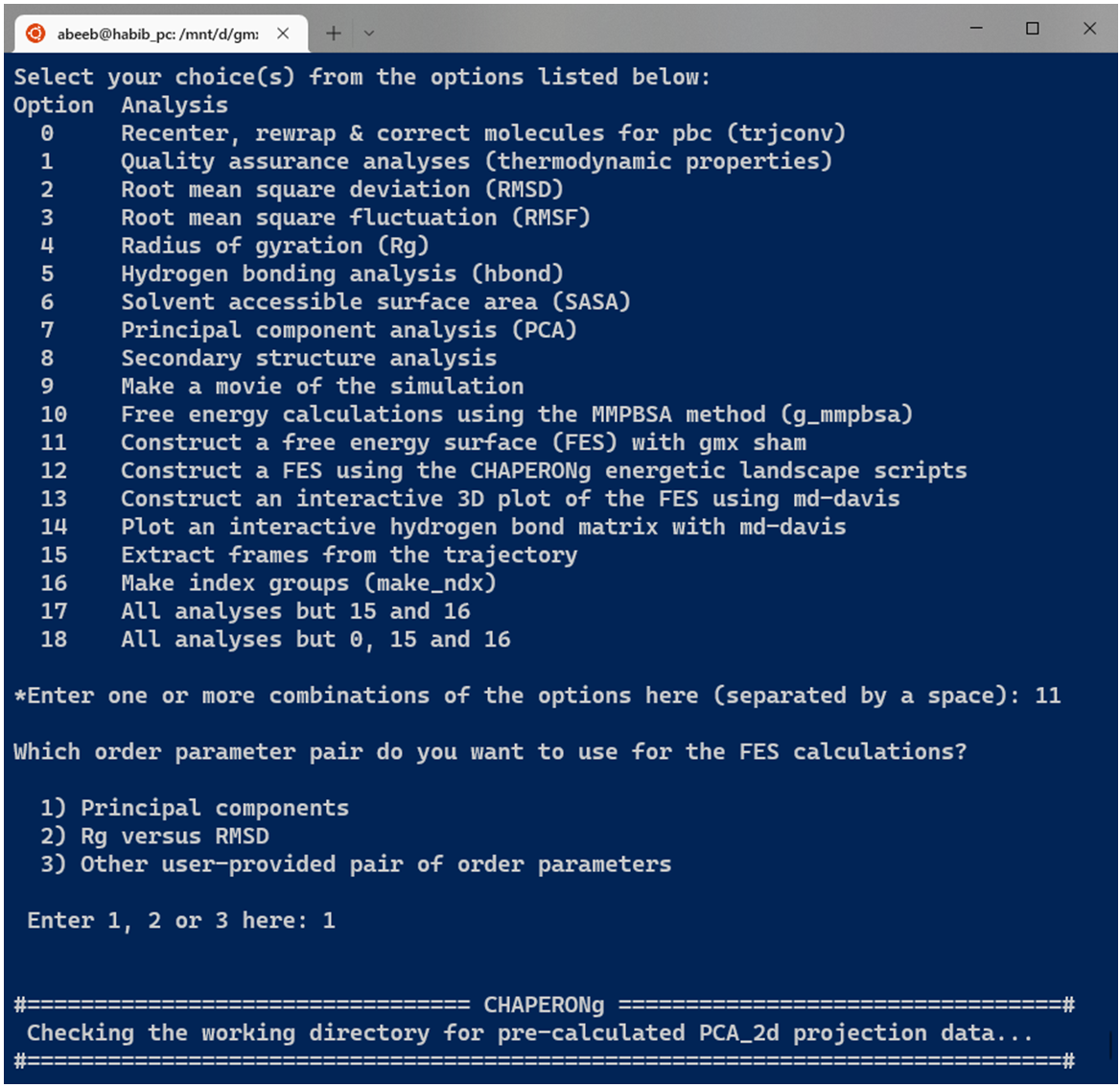
Before running the FES calculations, the user is prompted to specify the type of input order parameters from preset options or some other user defined parameters (see Image below). One preset option is to directly use the .xvg plot of the projection on the first two eigenvectors from PCA obtained with GMX. If chosen, CHAPERONg checks the working directory for a previously run PCA folder. If found, the PCA_2Dproj.xvg file is automatically used. If no such directory or file is available in the working directory, the process is rather initiated with a PCA run. When a precalculated PCA result is avaiable, the FES calculation is automatically run if CHAPERONg is launched in the full auto mode. But if launched in the semi-auto mode, the user is asked to confirm whether to use the pre-calculated PCA_2d projection file, repeat PCA calculation, or provide some other PCA_2d projection file located in some other directory.

12.2. Rg Vs RMSD FES with gmx sham

Similar to the case of the PCA-derived FES, a second preset option is to use the Rg and the RMSD as the quantities of interest (order parameters).

12.3. Outputs of the FES calculations with gmx sham

Using the gmx sham tool, the Gibbs free energy.xpm file is generated, which is a matrix file that contains the plot of the estimated relative Gibb’s free energy of the system at different states/conformations in the energetic landscape. Other output files are also generated such as:

• prob.xpm: a matrix plot of the probability of the system being in a particular conformation at a particular point in the free energy landscape,
• bindex.ndx: a list of the different bins of the 2D histogram and the trajectory frames that make up each bin,
• shamlog.log: a list of the lowest energy bins, their estimated relative free energy values, and the index of each bin as contained in the bindex.ndx file.

12.4. Extracting (low-energy) structures from the trajectory

Following the FES calculations, three representative structures are extracted, in the order in which they exist in the index list, from the lowest energy bins. Afterwards, the user has the option to extract additional structures of their choice by providing the frames of the structure to be extracted, perhaps guided by the information available in the shamlog.log and the bindex.ndx files.

13. FES using the CHAPERONg energetic landscape scripts

13.1. A 2D representation of the free energy landscape

Free energy surface (FES) in CHAPERONg is constructed using a previously described method (Tavernelli et al., 2003; Papaleo et al., 2009). To obtain a 2D representation of the free energy landscape, the Boltzmann inversion was used to calculate the free energy as shown in the equation (10) below:

$$ \tag {10} \pmb {{\Delta}G_{i}} = -kT\ln\left(\vcenter{\hbox{$\dfrac{P_{i}(r)}{P_{max}(r)}$}}\right) $$

where,

• $ k $ is the Boltzmann constant,
• $ T $ is the simulation temperature,
• $ P_{i}(r) $ is the probability of the system being in a particular state $ i $ characterized by some reaction coordinate $ r $ (quantities of interest) and is obtained from the size of the conformations in the histogram bin representing the state,
• $ P_{max}(r) $ is the probability of the most populated bin (i.e. most probable state), and
• $ {\Delta}G_{i} $ is the free energy change of the state $ i $.

Using the expression above, the relative free energy of the most probable state is computed to be zero, while other less probable states would have positive relative free energies.

13.2. Input quantities of interest

To construct the FES with CHAPERONg, the user is prompted to specify the input “order parameters”, similar to that seen in the Figure above. Several global parameters can be used to describe the free energy landscape (FEL); examples include the number of hydrogen bonds, RMSD, radius of gyration, or fluctuations along principal components, etc. To obtain a 2D representation of the FEL, two preset order parameter options are provided in CHAPERONg, including the 2D projection of principal components from a PCA and a RMSD-Rg pair. A third option allows the user to specify other input quantities of interest. Then, the indicated input quantities of interest are located in the working/specified directory and pre-processed. The construct_FES.py script is run on the data to estimate the optimal number of bins to be used in generating a 2D histogram of the data. Multiple estimators are used in deducing the number of bins, including the Freedman-Diaconis (1981), the Scott(1979), the Rice (1944), and the square-root methods. These are expressed, respectively, in equations (2), (3), (4), and (5) described above. The estimated number of bins with each method is written to a file named binning_summary.dat.

13.3. Plotting the free energy surface

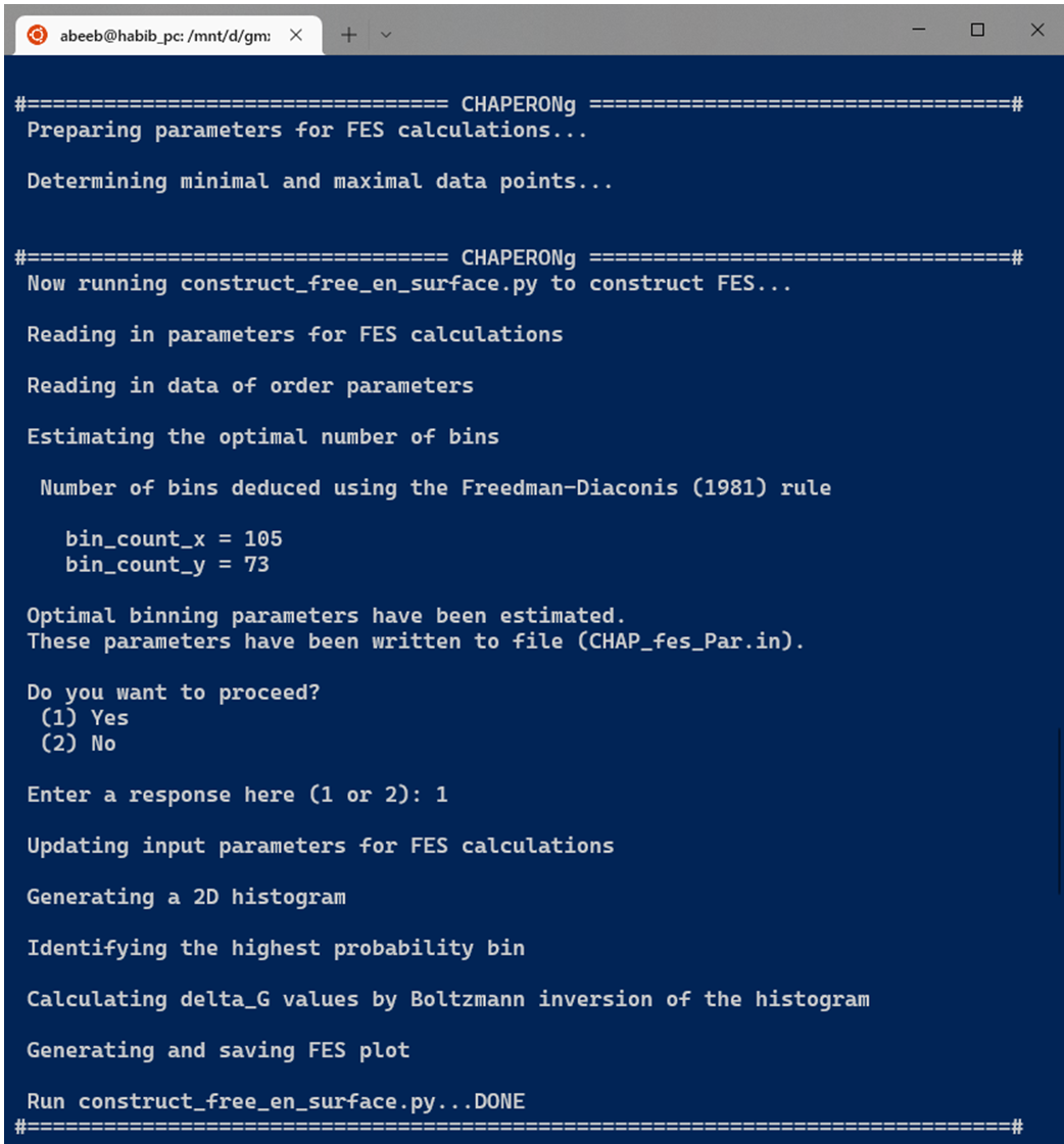
If CHAPERONg is run in the full-auto mode, the number of bins estimation deduced from the Freedman-Diaconis (FD) rule, as shown in the equation above, is automatically used for generating the 2D histogram because it is robust and takes into account data variability and size. But when run in the semi-auto mode, the user is prompted to confirm whether to proceed with the FD estimation of the number of bins. When principal components are used as the input order parameters, a default of 100 bins in each of the two dimensions is set (this value was found to work out well in all tested cases). At this point, the user may decide to replace the bin count parameters and/or order parameters in the generated input parameter file CHAP_fes_Par.in in the working directory. Using the input data and parameters, the 2D histogram is generated and used in estimating $ {\Delta}G_{i}$ by Boltzmann inversion as described above. Then, the FES is plotted and saved as a PNG figure.

13.4. Extracting (low-energy) structures from the trajectory

After the FES is generated, the user is prompted to decide if the lowest energy structure should be extracted. To achieve this, the landscape parameters are mapped to the simulation time using the CHAPERONg script map_fes_parameter_to_simTime.py. The corresponding time for the lowest energy structure is identified using the CHAPERONg script get_lowest_en_datapoint.py and then passed to the gmx trjconv module to extract the structure. To allow the extraction of other user-chosen structures based on the free energy, the user is prompted whether to proceed with mapping all the data points from the free energy surface to their corresponding simulation time using the CHAPERONg scripts map_all_dataPoint_to_simTime.py and approx_dataPoint_simTime_for_freeEn.py. The files generated can then be used to guide the choice of structures to be extracted from the trajectory.

14. Interactive 3D FES using md-davis

The construction of a 3D plot of the FES, enabled by the md-davis tool, is similar to those described above. Two preset input order parameter pairs are provided, including the principal components, and RMSD-Rg. A third option lets the user specify some other quantities of interest to use. However, the md-davis functionality is only available if:

• CHAPERONg has been installed via the conda installation option, OR
• you have installed md-davis in a seperate environment and then launch CHAPERONg from that environment.

For details of how md-davis generates the energy landscape, you can read the relevant part of its documentation here. An output plotly-generated .html file is produced which, when opened in a browser, shows an interactive 3D plot with several control buttons, including an option to save the plot as a .png image.

15. Interactive Hydrogen Bond Matrix Using md-davis

The construction of an hydrogen bond matrix is also achieved with the aid of md-davis, which analyzes the hydrogen bond data produced by gmx hbond. md-davis uses the GROMACS output .xpm matrix data to produce an interactive plot that gives detailed information about the hbond contacts recorded in the trajectory. You can find more details in the relevant part of the md-davis documentation. To implement md-davis, CHAPERONg first calls GROMACS to extract a reference structure (the first structure from the trajectory) to be used by md-davis. Then the hydrogen bond list is extracted from the GROMACS output index file. These files are then passed to md-davis to produce an html plot containing the detailed interaction matrix. The html and other output files are saved in a subfolder hbond_matrix in the working directory. In the current version of CHAPERONg, the occupancy cut-off for the hydrogen bonds displayed in the plot is set to 33 %.

16. Average of Replica Analysis Plots

Often times, MD simulation is often conducted as multiple replicas of the same system and the trajectories analysed as means of the replicas. This not only enables a wider sampling of the conformational space but also provides more statistically reliable data, improved reproducibility and error estimates. The calculation of the average of such replica plots can be carried out easily with CHAPERONg. This requires the user to specify the path to the directory containing the input .xvg replica plots by using the --path_av_plot flag or by providing the corresponding parameter in the paraFile.par file. In addition, the user can specify a label (RMSD, RMSF, Rg, SASA, hbond, etc.) for the input files using the --data_label parameter. Otherwise, the user would be interactively prompted to provide this during the run.

I try my best to make the information on this website as accurate as possiblef you find any errors in the contents of this page or any other page on this website, I would greatly appreciate that you kindly get in touch with me at contact@abeebyekeen.com. Also, you are welcome to reach out for assistance and collaboration.