Automated MD Simulation Trajectory Analyses - Part I

Discover the myriads of post-simulation processing and analyses that CHAPERONg automates.

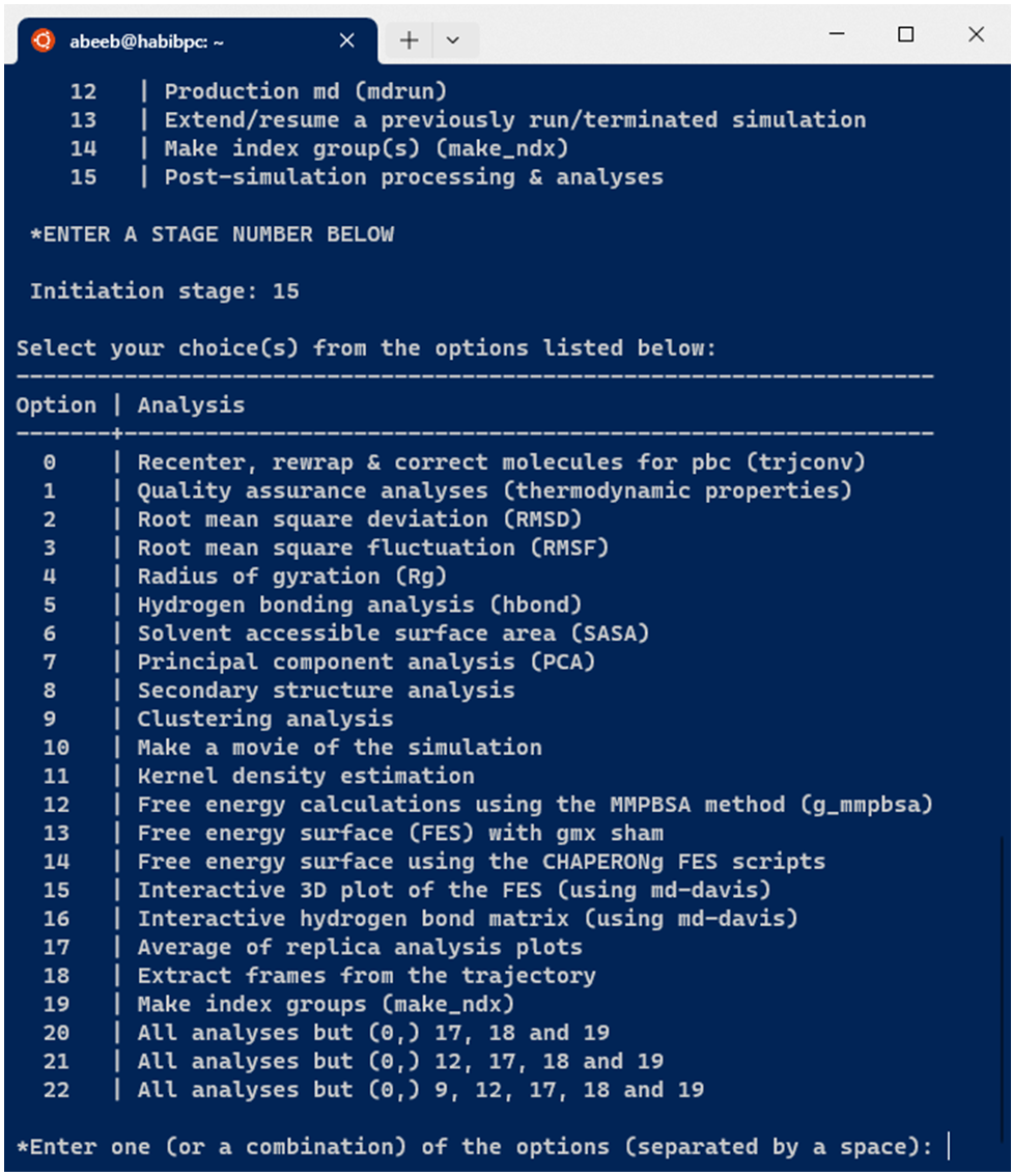
CHAPERONg integrates and automates up to 20 post-simulation trajectory processing and analyses (see Figure below).

1. PBC Correction

The simulation trajectory can be corrected for periodicity using the GROMACS trjconv tool. Several options are available and parsed to GROMACS to run trjconv. The user can provide the required option using the CHAPERONg inputtraj flag via the command line or specified in the paraFile parameter file. The available options including noPBC, nojump, center, fit, and combo are described below.

If no option is provided, CHAPERONg generates, based on the type of simulation, a suitable PBC-corrected files for use in the subsequent analyses. For protein-only (including protein-protein complex) systems, the noPBC is created. This noPBC file is used by default, but from experience, both the noPBC and nojump files work for one-chain protein systems; but the nojump file works better for protein-protein complexes. Hence, it is recommended that the user supplies the appropriate option accordingly. For protein-ligand systems, the center file is created and used when no option is specified by the user.

2. Quality Assurance Analyses

This option carries out analyses of some thermodynamic parameters similar to those quality assurance analyses described earlier for pre-production energy minimization and equilibration. The key difference here is simply the energy (.edr) file read; which in this case is the MD simulation energy file containing the energy terms and thermodynamic parameters collected during the simulation. The plots of the thermodynamics parameters and their generated finished figures are saved in a postMD_thermodynamics folder.

3 RMSD, RMSF and Rg

The computation of the root mean square deviation (RMSD), root mean square fluctuation (RMSF), and radius of gyration (Rg) are automated by CHAPERONg. These are respectively based on the corresponding GROMACS modules gmx rms , gmx rmsf, and gmx gyrate . You can visit the linked GROMACS documentation pages for details of the calculations performed by each of the modules. For each of these analyses, if the results folder of a previous run is detected in the working directory, CHAPERONg backs it up as, e.g., RMSD#.backup.1, or #RMSD.backup.2, etc., depending on the number of previous runs.

4. Hydrogen Bonding Analysis

The number of hydrogen bonds between the protein atoms or between the protein and water atoms (in the case of a protein-only system) is calculated using the gmx hbond tool. In the case of a protein-ligand system, the number of hydrogen bonds between the protein receptor and the ligand is also calculated. In addition, the hbond matrix and the hbond index files are also generated using the -hbm and -hbn options. These files are required for generating the interactive hbond matrix with MD-DaVis program (discussed below under the MD-DaVis-enabled hbond matrix plot).

5. Solvent Accessible Surface Area

The calculation of the solvent accessible surface area of the protein is run with gmx sasa, and both the XVG plot and the PNG image file are saved in a SASA folder in the working directory. If the results folder of a previous run is detected in the working directory, CHAPERONg backs it up as #SASA.backup.1, or #SASA.backup.2, etc., depending on the number of previous runs.

6. Principal Component Analysis

For the principal component analysis, also called the covariance analysis, the gmx covar module is first used to compute and diagonalize the covariance matrix to generate the named eigenvec.trr and eigenval.xvg files. Using the gmx anaeig module, these files are then used to analyze the eigenvectors (principal components) and calculate a 2d projection of the trajectory onto the eigenvectors. The plot of the 2d projection and related output files are saved in the PCA folder. Similar to other analyses, an existing results folder of a previous run is backed up as #PCA.backup.1, #PCA.backup.2, etc.

7. Secondary Structure Analysis

The secondary structure analysis on GMX is carried out by the gmx do_dssp module. The assignment of secondary structure relies on the DSSP program as a dependency. If you don’t have DSSP installed on your machine, you can download it from the DSSP website.

1

export DSSP=path/to/dssp

If the user has no DSSP installed, or the environment is not properly set, GMX fails to run secondary structure analysis. However, CHAPERONg has been packaged with a DSSP executable, and the user is prompted if this executable should be configured for use by GMX instead.

1

export DSSP="$(echo $CHAPERONg_PATH)/CHAP_utilities/dssp-x64"

Once a functional “DSSP” is available, the secondary structure is computed using the gmx do_dssp module. To calculate the secondary structure, the coordinates of the protein mainchain (without the sidechains) are used as these provide sufficient data for the assignment of the secondary structure elements by DSSP. Depending on the duration of the simulation, the secondary structure will be recorded at e.g., every 0.5 ns (for a 50 ns simulation), 1 ns (for a 100 ns simulation), 2 ns (for a 200 ns simulation), etc. This reduces the computation time and also gives rise to a much clearer plot of the variation of the secondary structure elements of each residue against time.

The default DSSP produces the secondary structure plot with seven types of secondary structure elements. To simplify the appearance of the plot and also aid its visualization and analysis, CHAPERONg produces a second copy of the .xpm matrix plot modified to reduced the secondary structure elements to four basic types including helices, beta-sheets, turns and coils. This modified plot is then used to generate a .eps postscript file using the gmx xpm2ps module. The postscript file is then converted to a .pdf format using the ps2pdf program, which is commonly pre-installed on most linux distros. The postscript file is also used to generate an additional .png output file using the linux convert program. All the output files are saved into a folder named Secondary_structure.

8. Clustering Analysis

MD simulation can typically generate a lot of data that may be difficult to handle and analyse–especially down to the little details. To facilitate a much easier handling and analysis of conformations from a simulation, the structures in the simulation trajectory can be clustered to identify and group together sampled structures that are similar. The gmx cluster module offers the functionality to achieve this, and is fully automated by CHAPERONg. Several clustering methods are available and supported by GROMACS; including the gromos (Daura et al., 1999), linkage, Jarvis-Patrick, Monte Carlo and diagonalization methods. The choice of method can be specified using the --clustr_methd input flag to CHAPERONg via the terminal or the paraFIle.par parameter file. Other parameters that can be set are the following:

• --clustr_cut: RMSD cut-off (in nm) to determine structure neighbours and cluster membership.
• --frame_beginT: Time (in ps) of the first frame to read from trajectory.
• --frame_endT: Time (in ps) of the last frame to read from trajectory.
• --dt: Time interval (in ps) at which frames are taken from trajectory.

The backbone atoms are used for least squares fitting and RMSD calculation. The output files are saved in a folder named Clustering and contain the following:

• clustering_details.log: Details of the clustering run including the method and RMSD cutoff used, the number of structures, and the number and list of all the clusters and their populations.
• clusters_representatives.pdb: All representative structures from the different clusters.
• cluster_id.xvg: A plot of the cluster number as a function of time.
• cluster_size.xvg: A plot of the cluster sizes.
• clusters_rmsd_distribution.xvg: An histogram of the RMSD distribution.
• clusters_index.ndx: A list of the indexes of the frame numbers and the corresponding clusters to which they belong.

9. Simulation Movie

9.1. Number of frames

To make a movie of the simulation trajectory, the total number of frames in the trajectory can be summarized into a smaller number of frames extracted at regular intervals. This number can be specified using either the --movieFrame at the launch of CHAPERONg, or provided in the parameter file paraFile.par. If the movieFrame parameter is not provided, the user is prompted to indicate whether a default 200-frame movie should be made or a different number of frames is desired. CHAPERONg uses PyMOL to create snapshots of the frames. Depending on the computing power of the user’s machine, it is generally better to not use more than 500 frames to avoid crashing of PyMOL due to overload.

9.2. Generating movie

First, CHAPERONg calculates the number of frames to skip at intevals in the trajectory based on the specified total number of frames. The resulting smaller trajectory is saved as a .PDB ensemble and then loaded onto PyMOL to extract the snapshots and render them as images. CHAPERONg checks if the convert program from the ImageMagick software is available on the device to produce high quality .GIF and .MP4 movies. This program is often generally pre-installed on most Linux distributions. If, however, a functional convert program is not detected (either because it is not installed, or a required library is missing), CHAPERONg then re-invoke PyMOL to instead use the mpeg_encode program (that is commonly available in PyMOL installations) to produce a .MPG video.

9.3. Handling previous runs

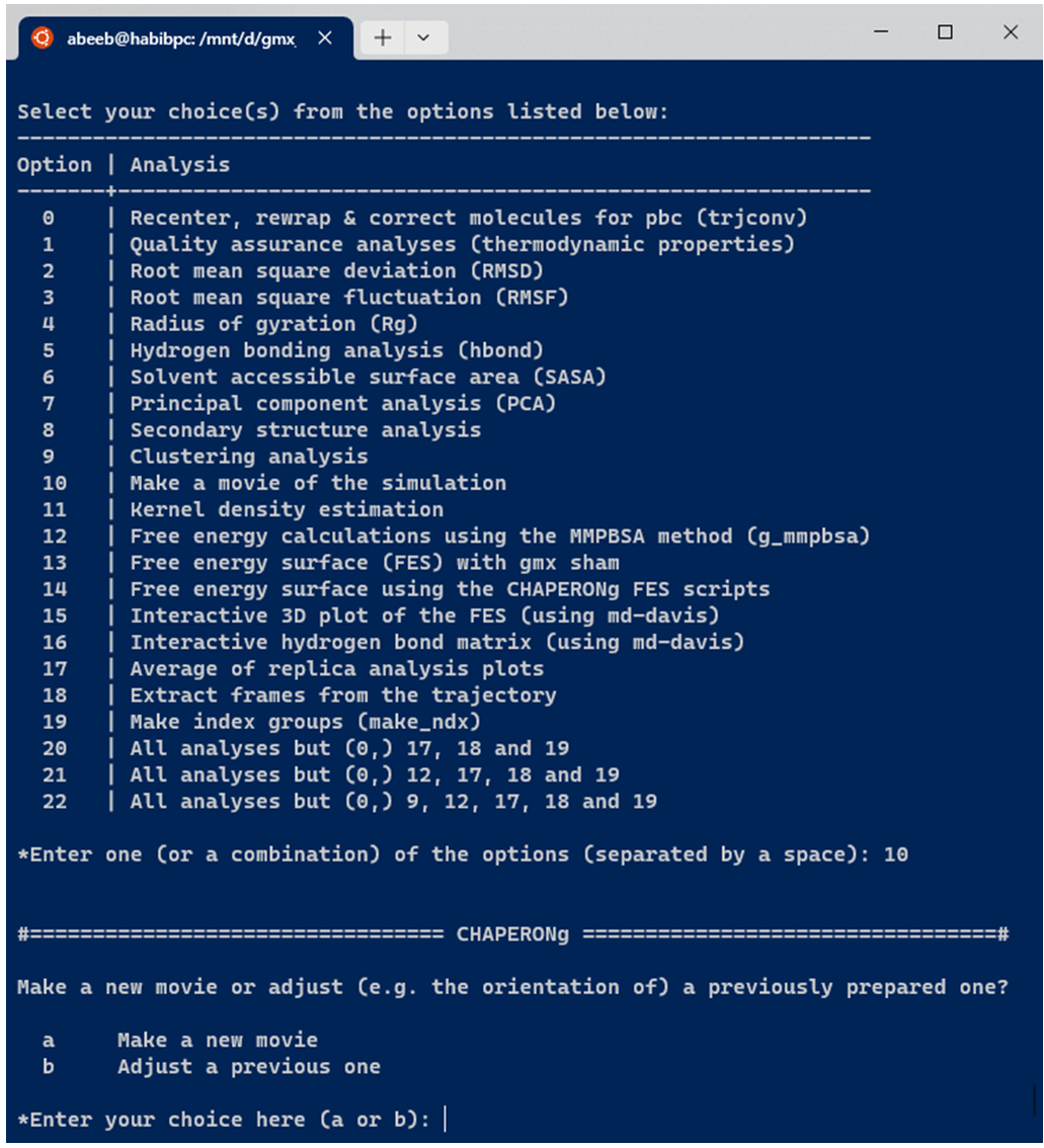
If the working directory contains a previously run MOVIE analysis folder, the previous run is backed up as a #MOVIE.backup.1, or #MOVIE.backup.2, etc., depending on the number of previous runs. If the user launches the movie creation as a single analysis and not as part of a workflow with other preceding or subsequent post-MD analyses, CHAPERONg checks the working directory for the existence of a previously run MOVIE analysis folder. If the result folder for such a previous run exists, the user is prompted to indicate whether the current run is to create a new movie or adjust (e.g. the orientation of) the previously made movie whose result folder has been found in the working directory (see Image below). Note that CHAPERONg only checks for the existence of the MOVIE folder and not necessarily the contents at this stage. So, an empty folder would give the same prompt.

9.4. Adjusting a previous runs

To adjust (e.g. the orientation of) a previously made movie, the user can change into the MOVIE directory, open the PyMOLsession_allSet.pse PyMOL session file, adjust the visual and save to update the session file. The the movie analysis can be rerun and CHAPERONg would locate the updated session file and use that to reproduce the movie. The movie from the previous run would be backed up before the new one is generated.

I try my best to make the information on this website as accurate as possiblef you find any errors in the contents of this page or any other page on this website, I would greatly appreciate that you kindly get in touch with me at contact@abeebyekeen.com. Also, you are welcome to reach out for assistance and collaboration.