CHAPERONg Tutorial 2
Automated MD Simulation of KEAP1 Kelch Domain in Water

A tutorial on how to use CHAPERONg for automated GROMACS MD simulation of a protein in water and post-simulation analyses.

0. Introduction

This tutorial follows up the previous tutorial where the use of CHAPERONg was briefly introduced. However, I mentioned over there that the first tutorial did not fully demonstrate the capabilities (and beauty 😊) of CHAPERONg—we only implemented the semi auto mode and the only post-simulation analysis that we carried out was to generate a movie. Using the flag -a full or auto_mode = full in paraFile.par, CHAPERONg can not only run the entire simulation pipeline in a fully automatic mode but also automatically carry out more than 17 post-simulation and trajectory analyses. In this tutorial, we will explore the capabilities of CHAPERONg to a much greater depth. We will carry out the MD simulation of the Kelch domain of the human KEAP1 (Kelch-like ECH-associated protein 1) in water. Like I previously mentioned in the first tutorial, if you haven’t performed MD simulation with GROMACS before (or any MDS at all), you may want to start with some basic tutorials to get familiar with the workflows and foundations of MD simulations and GROMACS itself. There are many excellent tutorials available such as those of Justin Lemkul, the Strodel Group, the Bonvin Lab, or those on the cgmartini website including the newer and older tutorials.

1. Preparing the Starting Structure

The starting structure of the human KEAP1 Kelch domain that we will be working with is the PDB entry (PDB ID) 4IQK. Download the coordinates file from the RCSB PDB. Crystal structures are often not without deficiencies. These include problems such as refinement inadequacies, as well as missing atoms and residues that could not be placed in the electron density. For researchers with the appropriate expertise, it is always a good and encouraged idea to inspect the electron density map of the structure of interest to ensure that the PDB model fits the density well enough, especially at regions of particular importance to the study. Fortunately, the 4IQK structure which we will be using in this tutorial is free from any major defects and can be directly used for MD simulation. If the structure you would like to use has missing atoms or residues, or has some other problems, click here to see the guide provided in Tutorial 1.

2. Cleaning up the Starting Structure

Copy the 4iqk.pdb structure that you have downloaded into a working directory where we will be carrying out all the subsequent actions of the simulation. Remove any undesired molecules in the crystallographic structure. Here, we will discard all the ligands (including the crystal water molecules) co-crystallized with the protein. This may not always be the best practice in all cases. However, for this tutorial, we are only interested in the apoprotein. Atoms of non-protein molecules (ligands and H₂O) in PDB structures are often labelled as “HETATM” (hetero-atoms). Enter the command below to clean the structure and write the coordinates of the KEAP1 Kelch domain apoprotein to the file KEAP1kd.pdb.

1

sed -E '/HETATM|HOH/d' 4iqk.pdb > KEAP1kd.pdb

Note that you can also achieve the above using any of your favorite visualizers (PyMOL, Chimera, Discovery Studio, Maestro, etc.). Simply save it into the working directory as KEAP1kd.pdb. A copy of the cleaned apo structure from the above command is available here.

3. Forcefield Files

GROMACS supports a number of forcefields which are available, by default, with GROMACS installations. The list and details of the supported forcefields, including AMBER, CHARMM, GROMOS, and OPLS, and their various distributions are provided in the relevant part of the GROMACS documentation. You can select and use the one that best suits your purpose. In this tutorial, we will be using the CHARMM36 forcefield, the latest version of which you can download from MacKerell Lab website. Download and copy the charmm36-***202*.ff.tgz file into the working diectory and run the command below to unpack the forcefield (note that the one used in this tutorial is the jul2022 version, which might not necessarily be the same for you by the time you are reading this):

1

tar xzvf charmm36-jul2022.ff.tgz

4. Define CHAPERONg Parameters

You can set CHAPERONg parameters—which control the inputs/ouputs passed to/from GROMACS runs—via one (or both) of two options:

1. You can configure the parameters into the CHAPERONg parameter file paraFile.par and pass it into the command that launches CHAPERONg. The paraFile.par file is present in the CHAP_utilities subfolder of the CHAPERONg package that you have downloaded/can download here. Alternatively, you can download a copy of the parameter file via this link. The paraFile.par contains self-explanatory comments.

2. You can specify the parameters as command line flags to CHAPERONg while launching it.

You can find more details about each of the parameters in paraFile.par by going through the relevant part of the CHAPERONg documentation.

5. Launching CHAPERONg

Before you run CHAPERONg, you need to copy all the required GROMACS MD simulation parameters files to the working directory. Name these files as:

• ions.mdp – mdp for the adding ions step
• em.mdp (or minim.mdp) – mdp for the energy minimization step
• npt.mdp – mdp for the NPT equilibration step
• nvt.mdp – mdp for the NVT equilibration step
• md.mdp – mdp for the production simulation step

You can click here to download a folder containing all the input files for the simulation we will be running in this tutorial. If you want to use these downloaded files, enter the commands below to extract the folder and cd into it:

1

tar zxvf chaperong-tutorial-2-keap1-kelch-domain-in-water-input-files.tar.gz

1

cd /chaperong-tutorial-2-keap1-kelch-domain-in-water-input-files

In the folder you will see a set of .mdp files and paraFile.par (the CHAPERONg parameter file for the simulation we will be running). The nsteps parameter in the md.mdp file is set to 50000000 so the simulation would run for 100 ns. You can reduce this value to a number that the computing power of your device can handle and complete within a reasonable running time. Open paraFile.par with a text editor to see what parameters have been set for the run. The command below launches CHAPERONg with the parameters in paraFile.par parsed to it.

1

run_CHAPERONg.sh -i KEAP1kd.pdb --paraFile paraFile.par

Note that the input starting structure is specified in the command with the -i flag. This is because that was not set in paraFile.par as you might have noticed. We could, alternatively, also launch CHAPERONg using the command below:

1

run_CHAPERONg.sh -i KEAP1kd.pdb -b cubic -T 12 -g -a full -p KEAP1kd -s tip3p -f wd --inputtraj noPBC -t 300 --movieFrame 250

The alternative command above achieves the same result as the one before it, except that the parameters were spelt out in the command rather than using the parameter file. The obvious limitation of the second approach is that the command is quite verbose and could get pretty long with more parameters, increasing the chances of errors and omissions. Note that you can also combine both approaches as convenient (I will demonstrate that later in this tutorial). However, when a parameter is specified both on the terminal and in paraFile.par, that of the terminal takes precedence over the one in the parameter file. After launching CHAPERONg, you will be prompted to choose the type of simulation (conventional or enhanced sampling) you wish to perform which is conventional in this case. Then choose protein-only as the type of system you would be simulating. Next, select the option that lauches the simulation from the first step (protein topology). The simulation will initiate and then proceed automatically till the completion of the production MD.

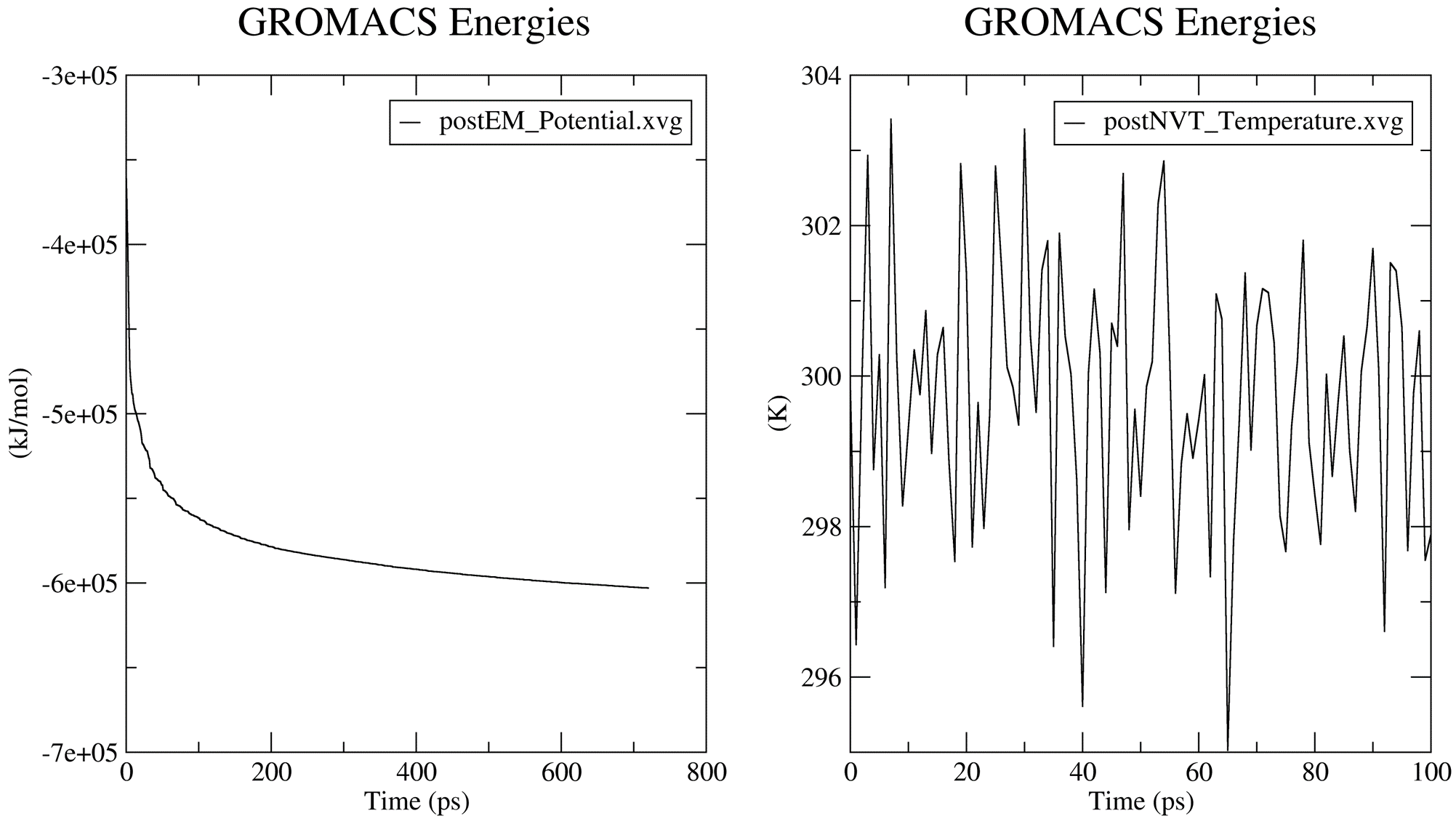
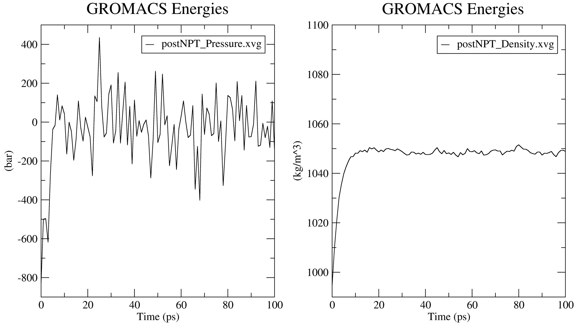
6. System Preparation Quality Assurance Checks

Prior to the production MD stage, CHAPERONg automatically carries out quality assurrance analyses by extracting some thermodynamic parameters—including the Potential Energy term upon the completion of the energy minimization step, and the Density, Pressure, and Temperature terms once the corresponding equilibration steps are completed. You can see more details about these in the relevant part of the documentation. The .XVG output of the plots and the .PNG images are saved in the working directory in a subfolder named postEM_thermodynamics. The figures generated are shown below. Note that for the post-minimization Potential energy plot, the output .XVG plot might need to be adjusted because the system started at a very high (large positive) state and quickly descended to a stable low negative potential. Thus, the first few (less than 10; 5 in this case) time steps have very large positive potential. This huge difference in potential betweeen the first few timesteps and the rest of the timesteps make the plot appear unnoticeable. You only need to adjust the extent of the Y-axis to make the plot more visible. The adjusted plot is presented in the figure below.

7. Post-simulation Trajectory Analyses

After the production run is completed, you will need to indicate whether to proceed to post-simulation analyses. Select yes and enter 21 to carry out all the analyses except g_mmpbsa Free Energy Calculation and Clustering. Since our simulation does not involve (inter-molecular) binding events, we won’t be running g_mmpbsa in the tutorial. We will however, run it in the next tutorial which involves a protein-ligand complex. As for Clustering, we would want to have an idea of what the trajectory looks like before we cluster structures from it. Because we set the auto_mode parameter to full in paraFile.par, all of the analyses will proceed automatically. Once completed, the result of each of the analyses will be saved in a corresponding subfolder in the working directory, named accordingly.

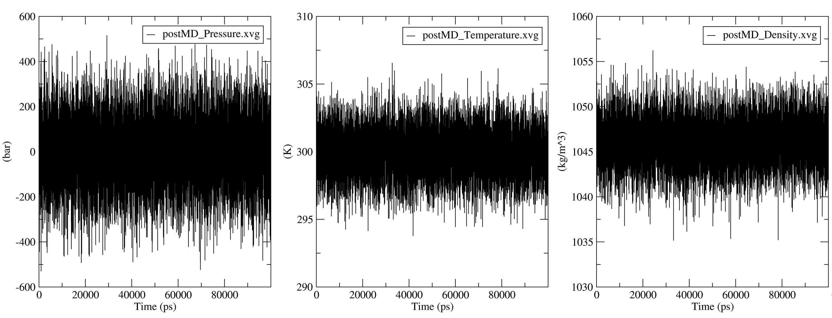
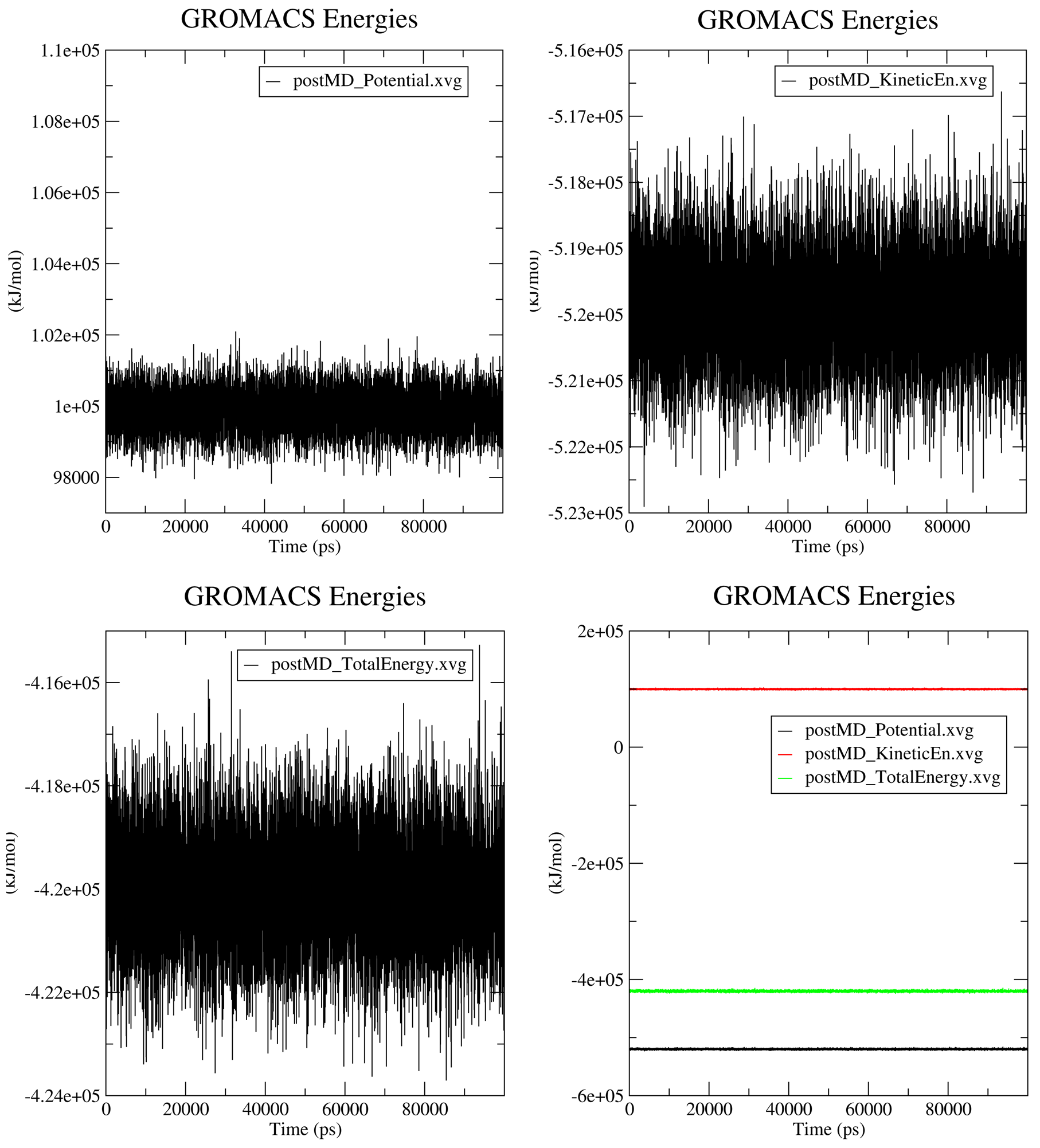
7.1. Progression of MD Thermodynamic Parameters

The thermodynamic parameters and energy terms collected during the simulation are automatically extracted and plotted using the gmx energy modules. The output .XVG plots and the generated figures are saved in a subfolder named postMD_thermodynamics.

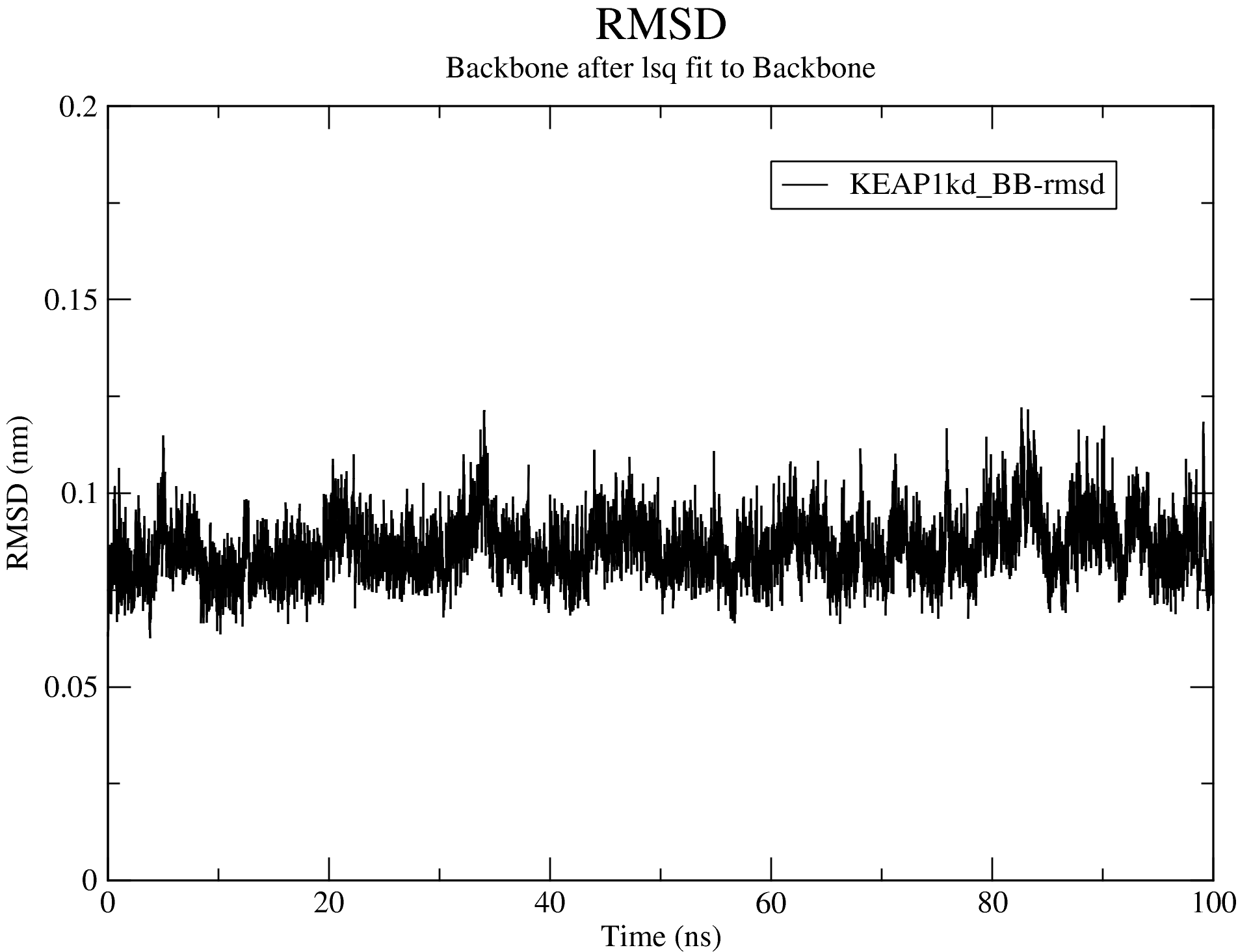
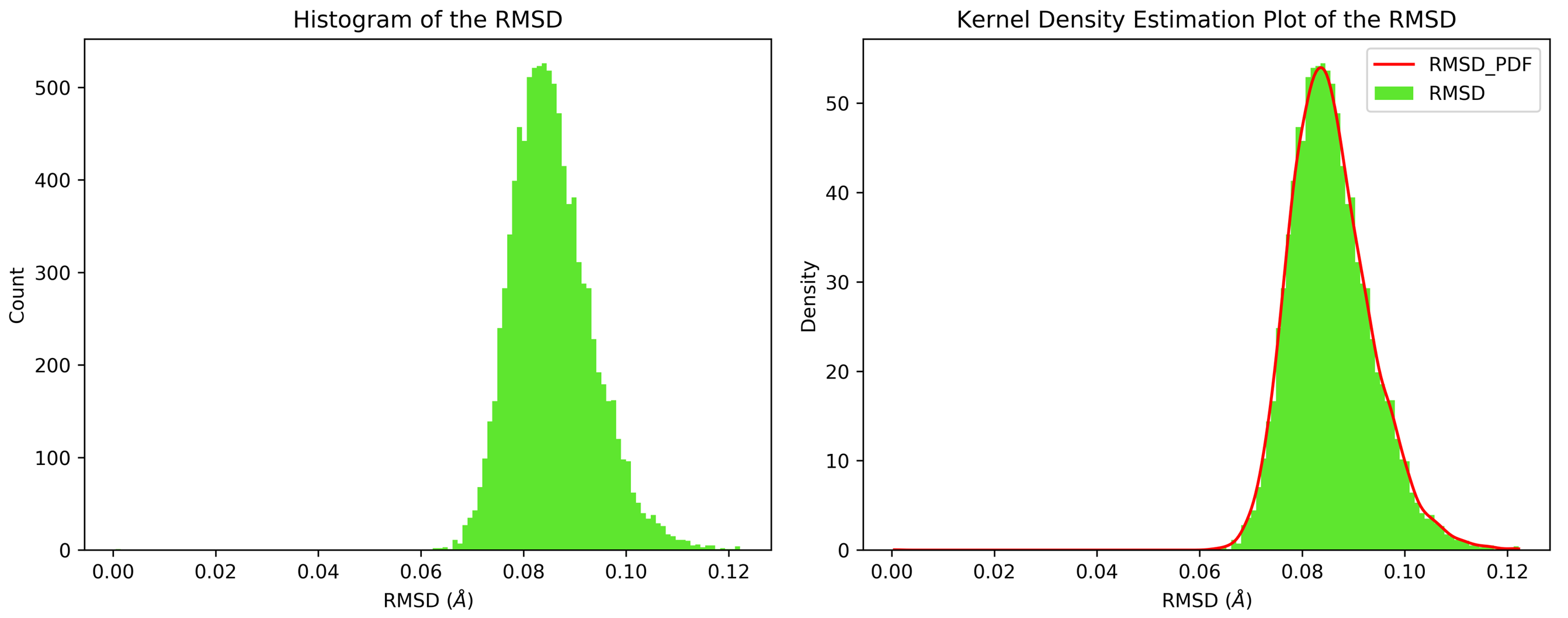
7.2. Root Mean Square Deviation (RMSD)

For details of the output produced for the RMSD calculations, see the RMSD section of the documentation.

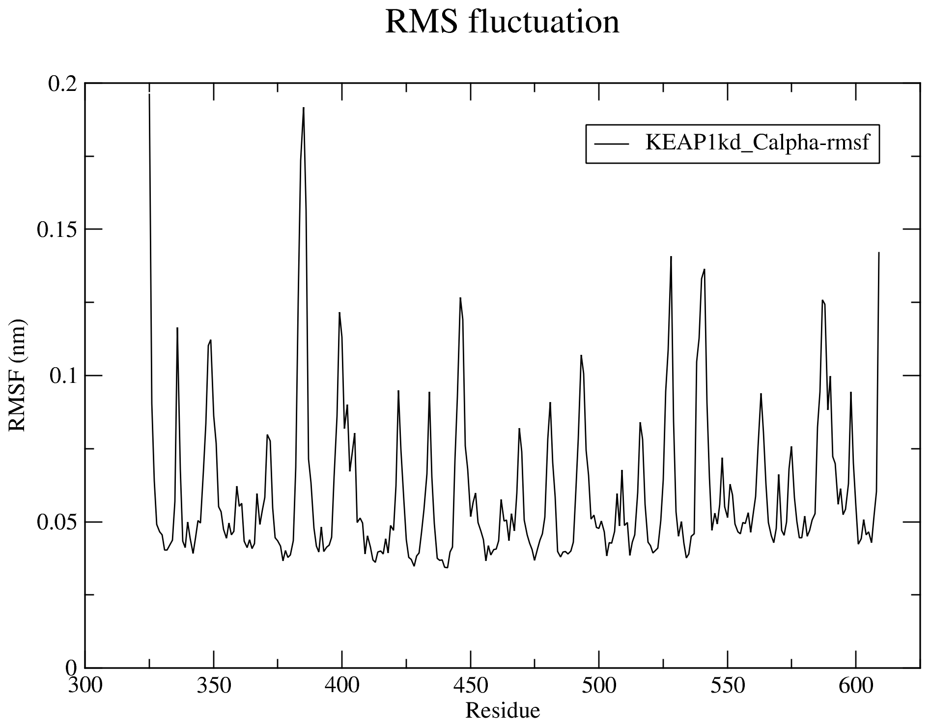
7.3. Root Mean Square Fluctuation (RMSF)

The RMSF can be likened to the b-factor (temperature factor) often obtained with crystal structures which is a measure of the residue level fluctuation of the structure. For more details, see the RMSF section of the documentation.

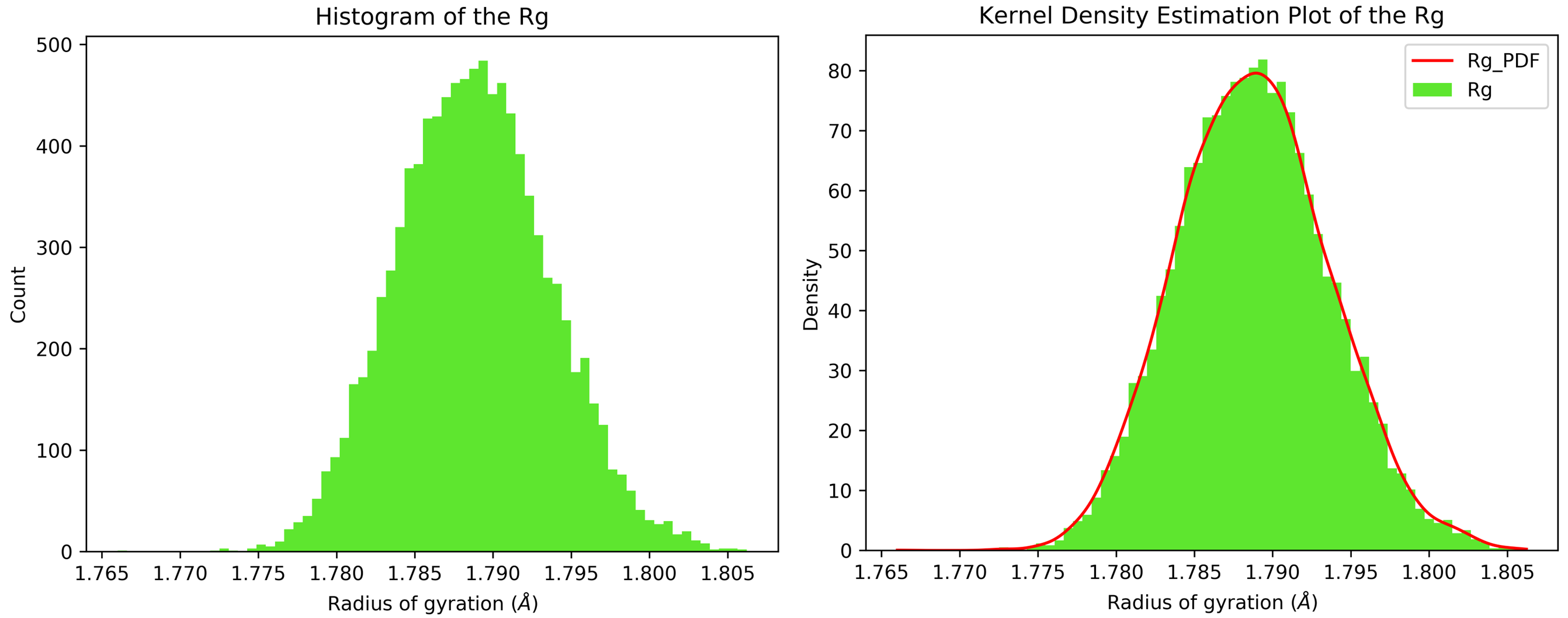
7.4. Radius of Gyration (Rg)

The radius of gyration plot produced by GROMACS has the time in ps unit. CHAPERONg converts the unit to ns to improve readability. For more details, see the Rg section of the documentation.

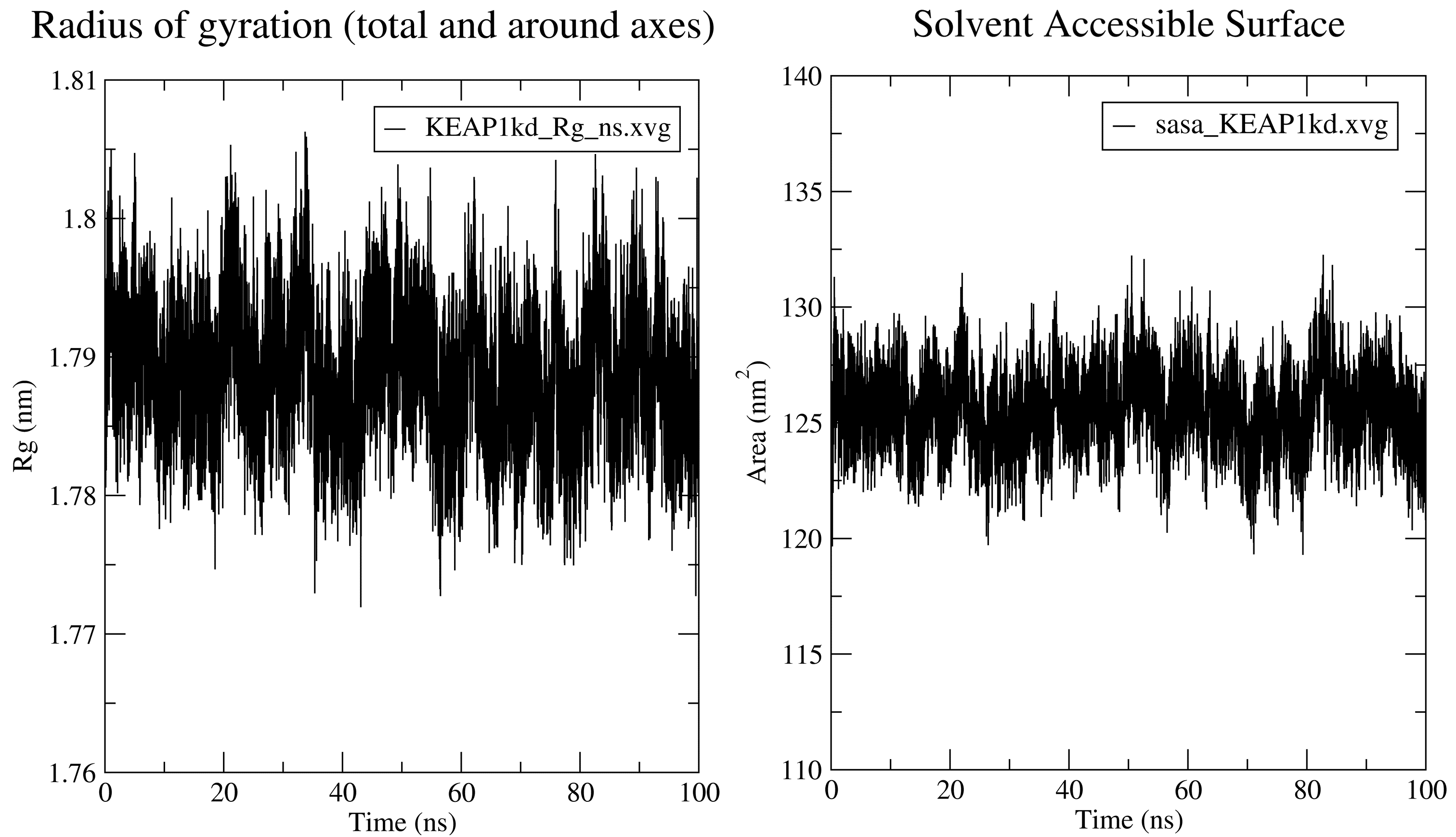
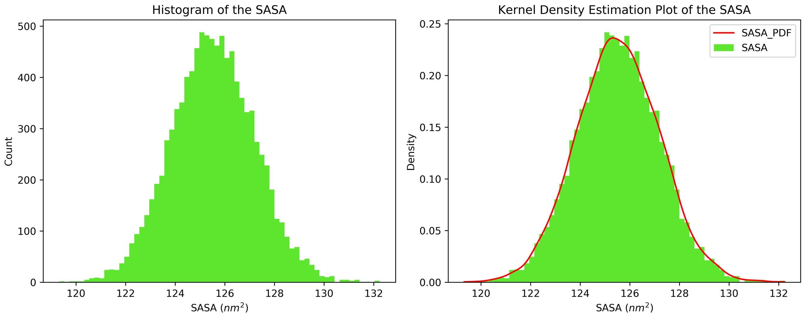
7.5. Solvent Accessible Surface Area

For details of what parameters are passed to GROMACS by CHAPERONg and a list of output produced and saved, see the SASA section of the documentation.

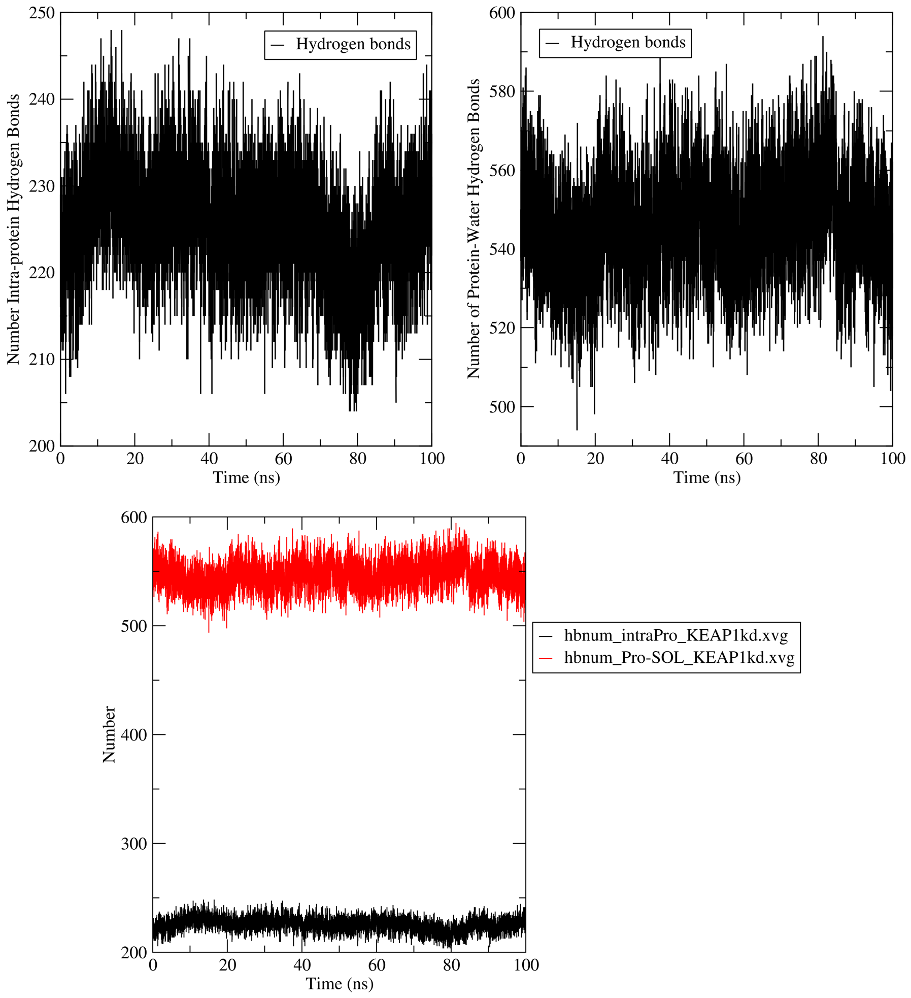
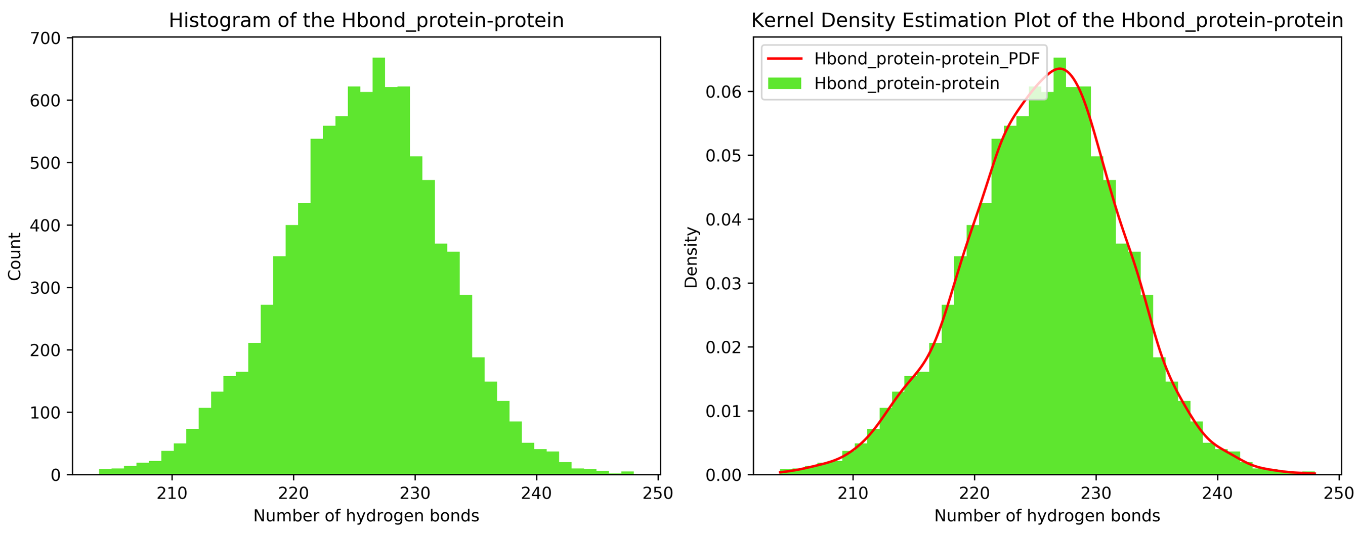
7.6. Hydrogen Bonding Analysis

Since the system simulated in this tutorial is protein-only, the hbond calculations passed to GROMACS by CHAPERONg include just protein-solvent hbonds and intramolecular (intra-protein) hbonds. For more details, see the hydrogen bond section of the documentation.

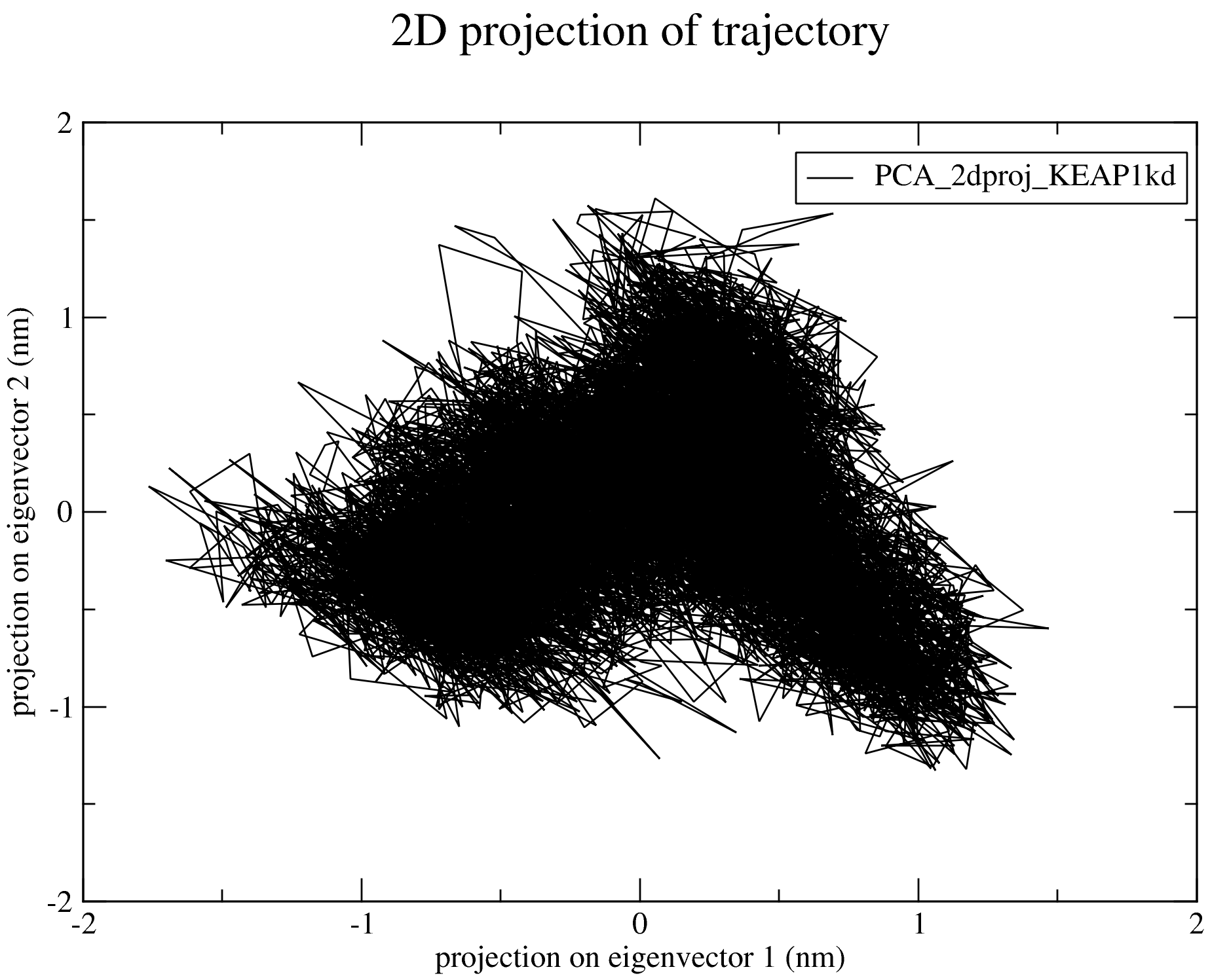
7.7. Principal Component Analysis (PCA)

Details and output of the PCA calculations are available in the PCA section of the documentation. Below is a 2D projection of the trajectory on the first two eigenvectors:

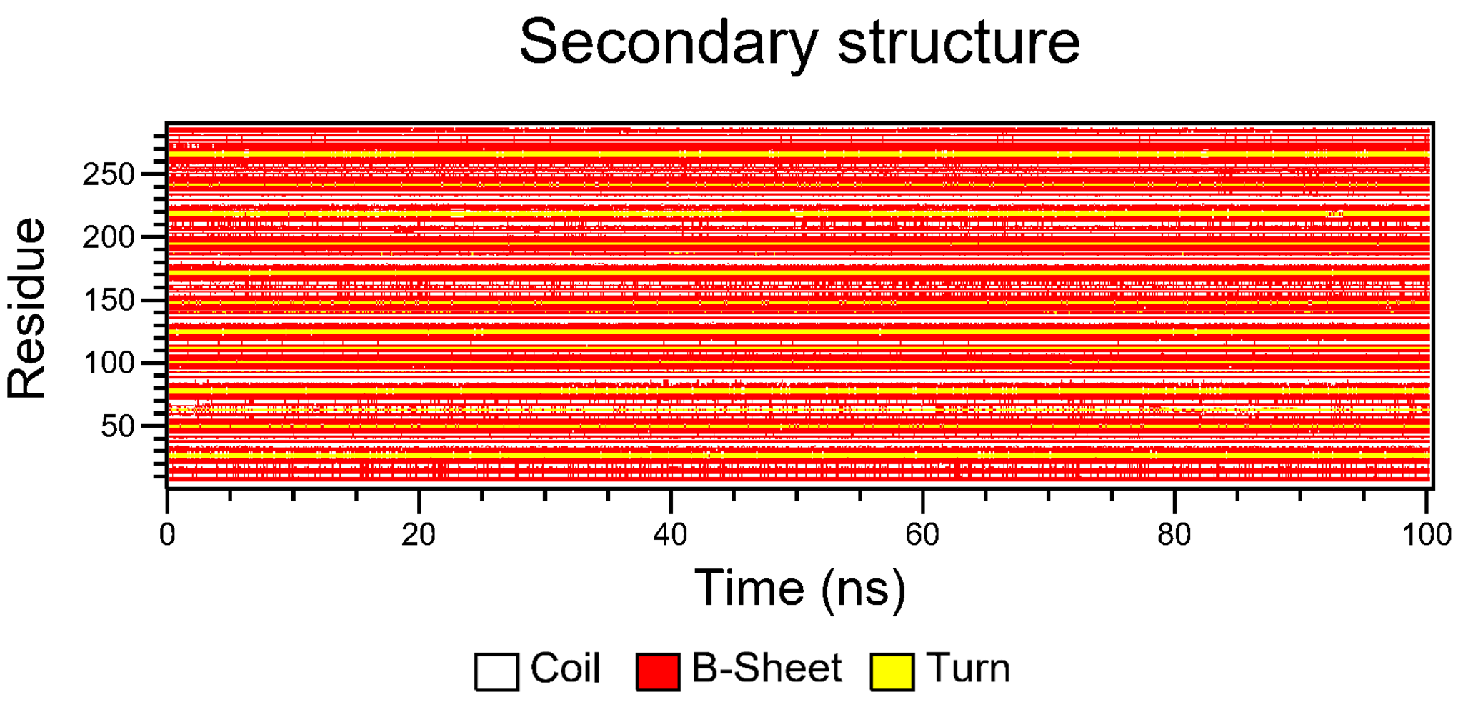
7.8. Secondary Structure Analysis

The details of how the secondary structures are computed and plotted are in the secondary structure analysis section of the documentation.

7.9. Clustering Analysis

Earlier, we skipped Clustering in our selection of the analyses to be automatically run by CHAPERONg. This is because we would typically want to have first a general idea of what the trajectory is like (by examining at the results of some of the trajectory analyses) to inform the decision of how we should carry out the clustering. Looking at the RMSD, Rg, and SASA plots above, we see that the system was quite stable and attained equilibrium right from the beginning of the simulation (post-NVT and -NPT equilibrations), which was maintained all through the simulaton time. Hence, we set the frame_beginT parameter in paraFile.par to 0 (ps) to consider all frames recorded during the simulation. Using the gromos clustering method (Daura et al.1999), the RMSD cut-off for two structures to be considered as neighbours was set to 0.085 (using the paraFile.par parameters clustr_methd and clustr_cut, respectively). This cut-off was chosen after multiple trials to see what value gave the best clustering results. This cut-off is that small because of the high stability of the system as you could see that the RMSD was mostly below 0.1 nm. You can update these parameters in your paraFile.par, or click here download a copy of the updated CHAPERONg parameter file (now named paraFile_updated.par for simplicity). Have a look at the parameter file and compare it with the previous one to see the difference. For more details of all the available options, see the clustering section of the documentation. To launch CHAPERONg for the clustering analysis, run the following command:

1

run_CHAPERONg.sh -i KEAP1kd_processed.gro --paraFile paraFile_updated.par

Or this (if you modified the previous parameter file):

1

run_CHAPERONg.sh -i KEAP1kd_processed.gro --paraFile paraFile.par

We could also choose to simply add the new parameters to the command without updating paraFile.par:

1

run_CHAPERONg.sh -i KEAP1kd_processed.gro --paraFile paraFile.par --frame_beginT 0 --clustr_methd gromos --clustr_cut 0.085

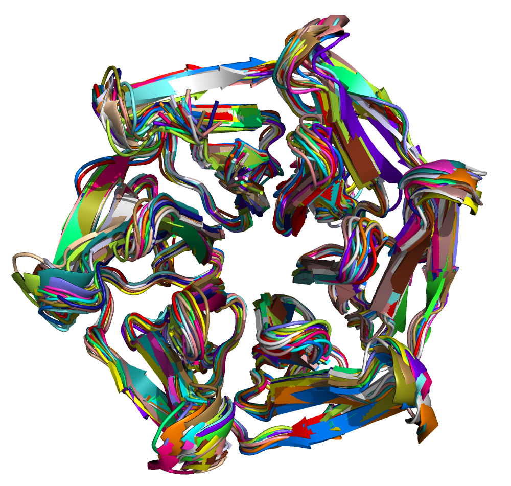
After the run is completed, the output files will be saved into the Clustering folder. The log file shows that, with the set cut-off, 24 clusters were identified and the representative structures for all the clusters are saved as clusters_representatives.pdb. The structures, superposed, are shown below:

7.10. Simulation Movie

The paraFile.par parameter movieFrame was set to 250 so that 250 frames are taken across the trajectory to generate a movie. For more details about simulation movie, see the relevant section of the documentation.

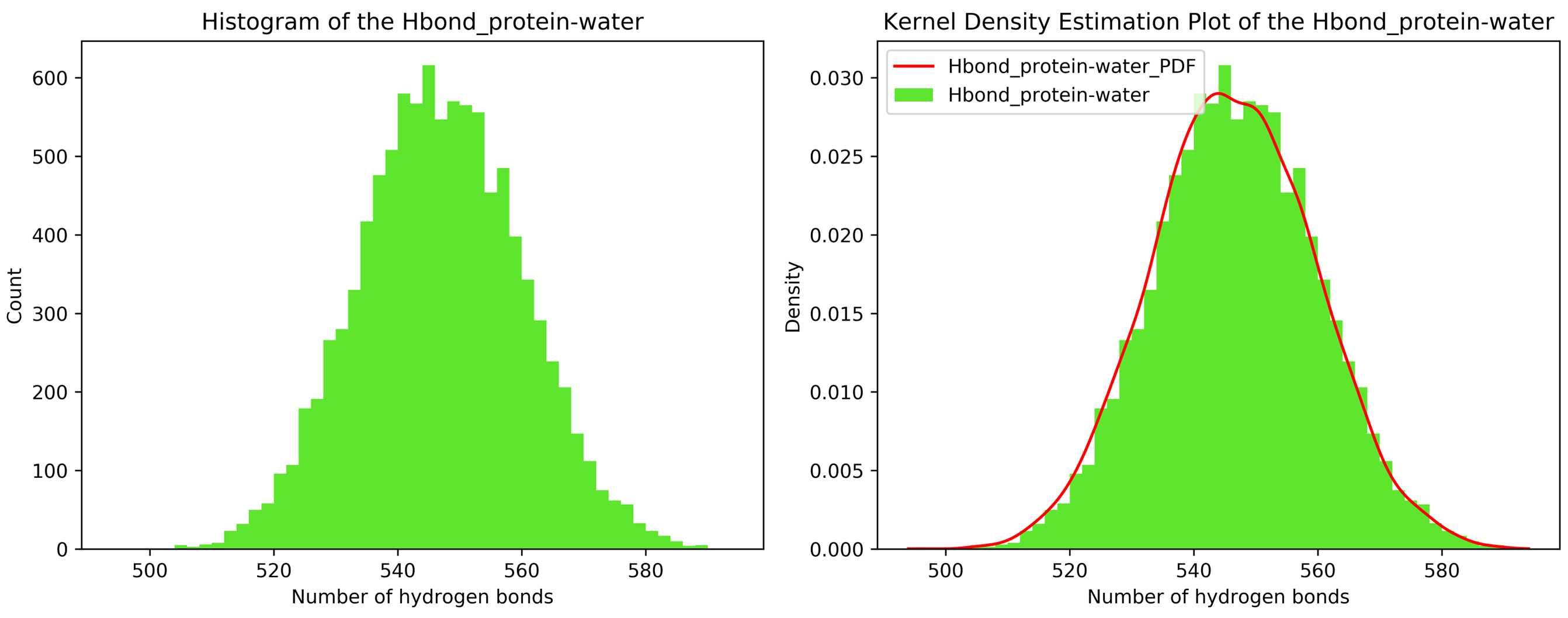
7.11. Kernel Density Estimation for Single Datasets

By running CHAPERONg in the full auto mode and selecting RMSD, Rg, hbond and SASA for KDE, the histograms and KDE plots for each of the specified data are generated. However, for some of the datasets in this tutorial, the automated estimation of the number of bins did not appear to be optimal. More optimal number of bins were then identified using the --kde_opt parameter of CHAPERONg (see the relevant section of the documentation for more details). The Xmgrace .XVG format of the plots are also generated. A file listing the statistics (the mean, the standard deviation, the minimum and the maximum data points, and the mode(s)—i.e. the most frequent values) of each data set is also generated.

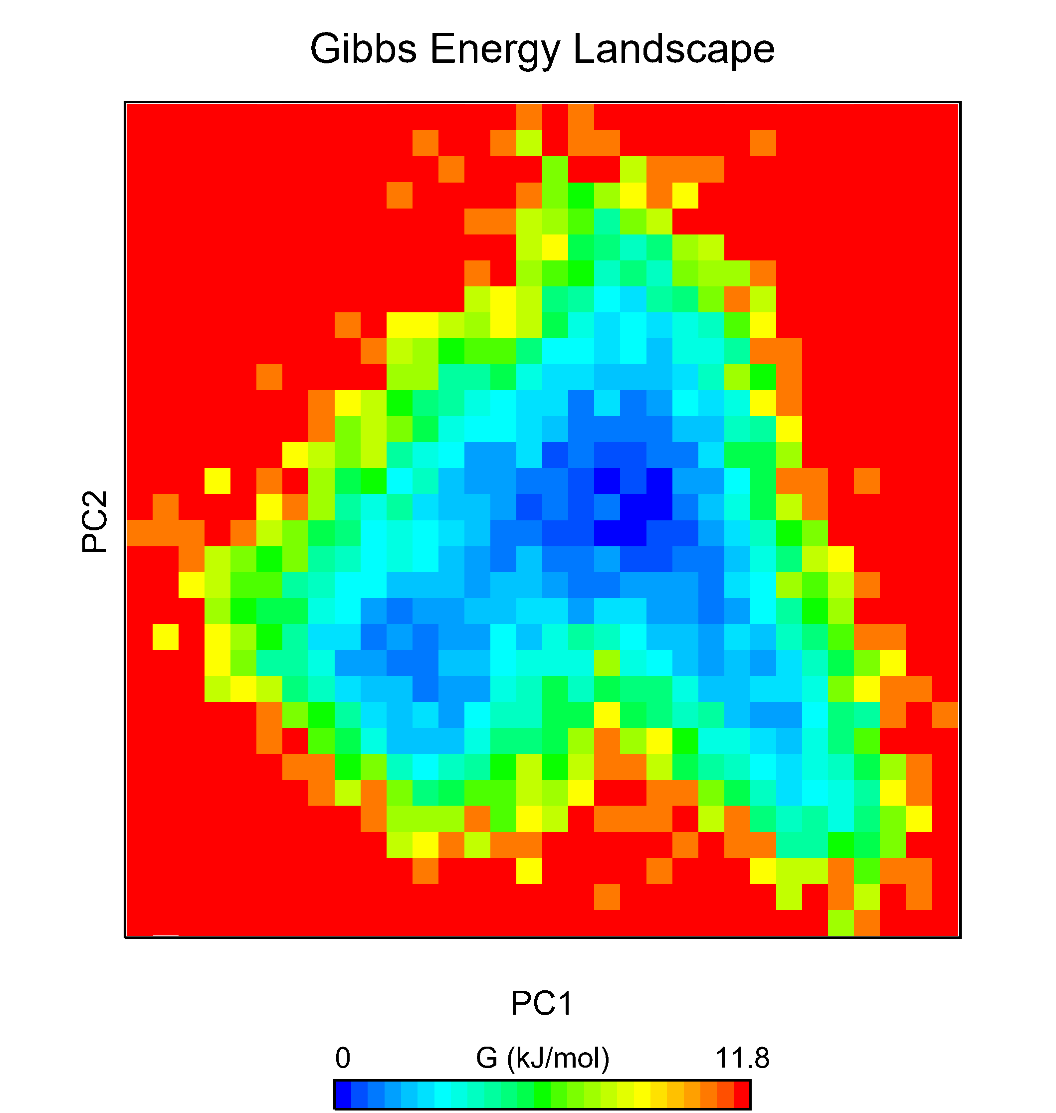
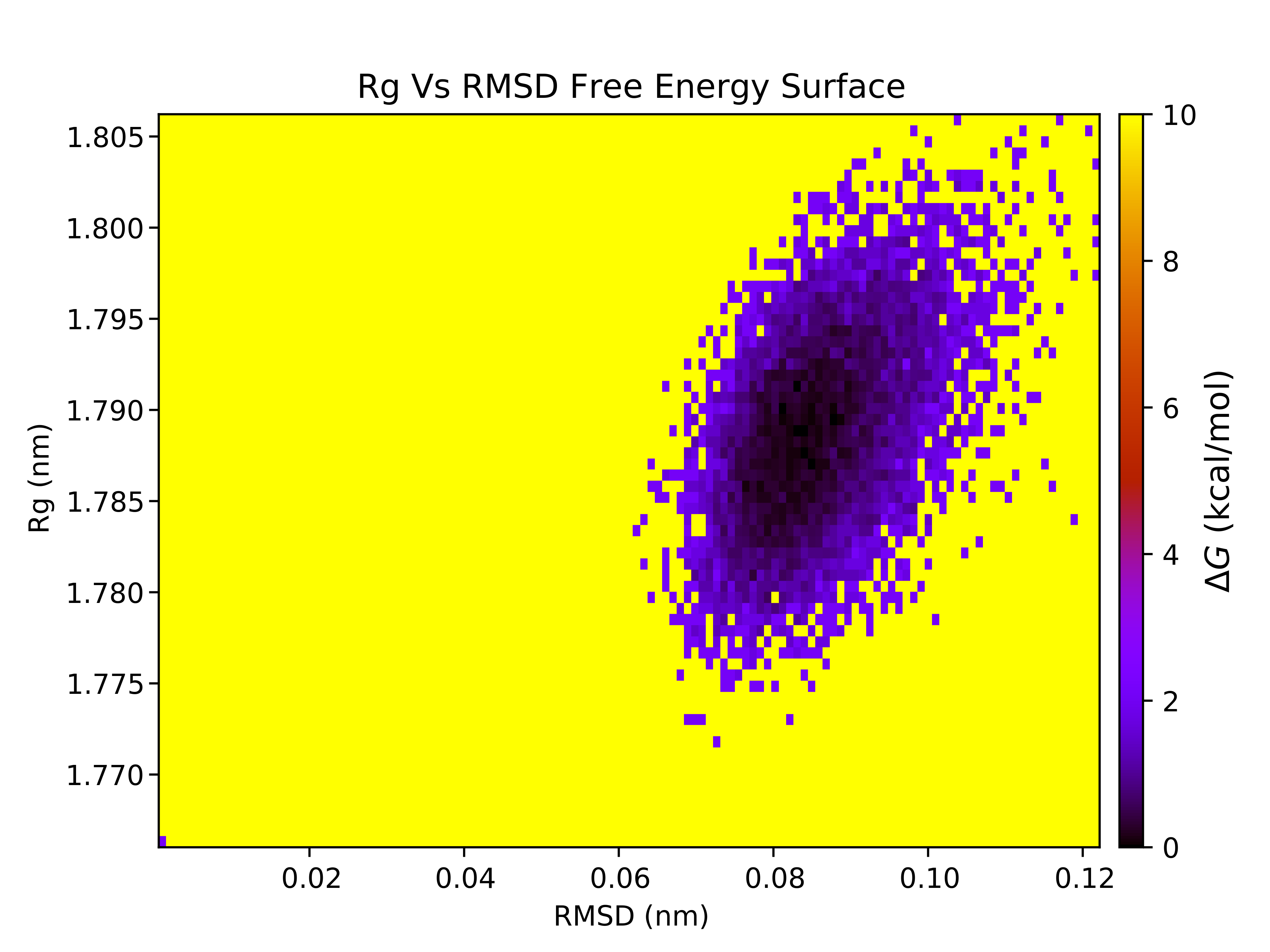
7.12. Free Energy Surface Calculations with gmx sham

The free energy surface (FES) of the trajectory can be constructed using several global parameters that describe the state of the system. With CHAPERONg, two preset options for the choice of order parameters are provided in addition to a third flexible, open option:

• Principal components from a PCA
• Rg versus RMSD
• Other user-provided pair of other parameters.

For illustration, below are the FES for each of the PCA-derived and RgVersusRMSD plots. If you are using data other than principal components, you may need to adjust the axes of the FES plots accordingly.

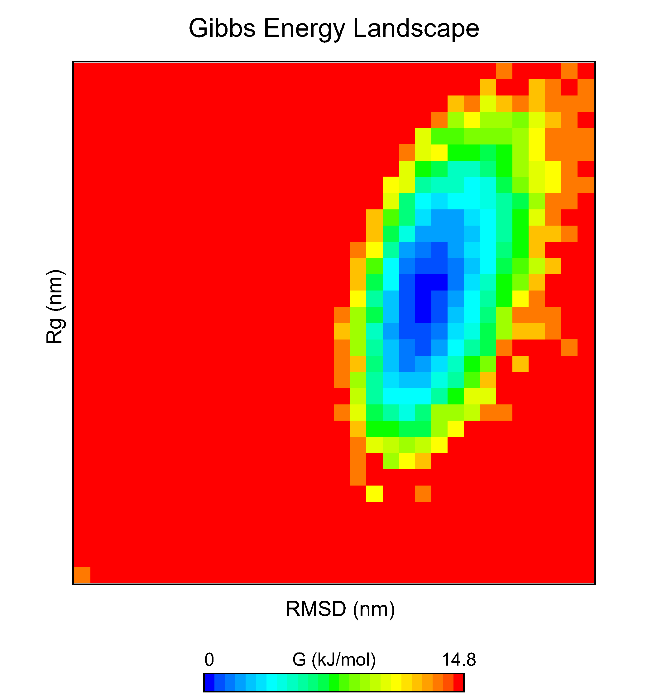
For each of the FES plots generated, three structures are extracted from the lowest energy bin. Much more can be done with CHAPERONg than this tutorial can cover. For example, by following through with the CHAPERONg prompts, you can choose to extract additional and specific structures from the trajectory based on their computed Gibbs free energy. You can find more details in the relevant section of the documentation.

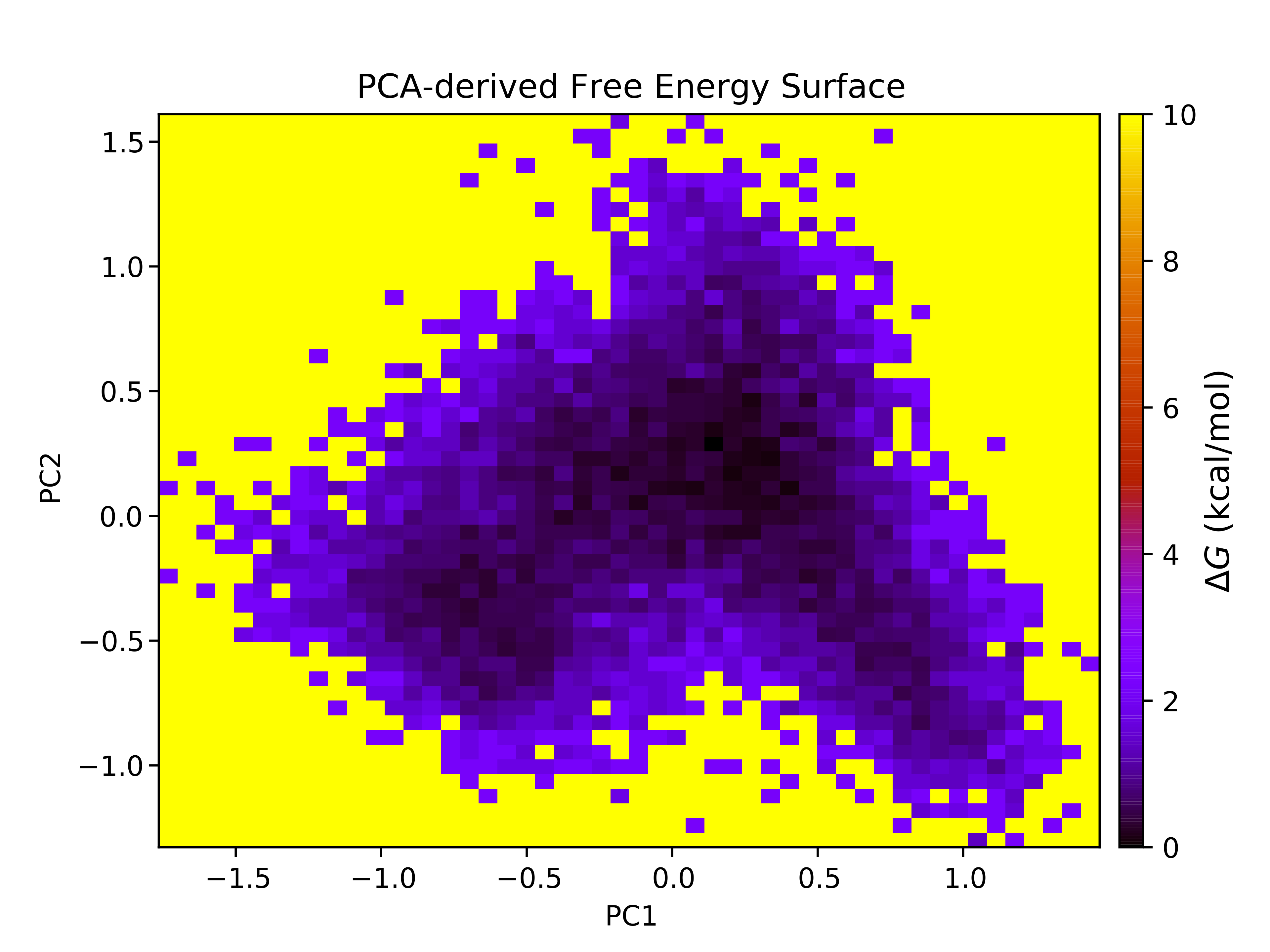
7.13. FES Using the CHAPERONg Energetic Landscape Scripts

Similar to the gmx sham module described above, the CHAPERONg FES scripts provide an alternative way to construct the FES.

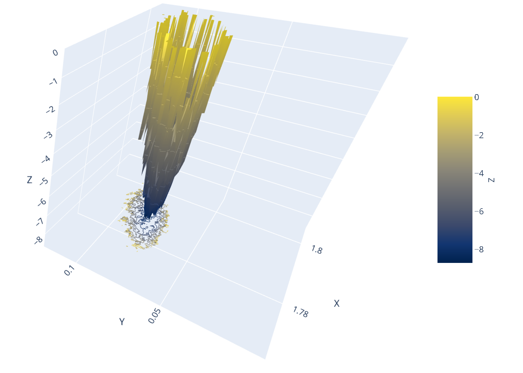
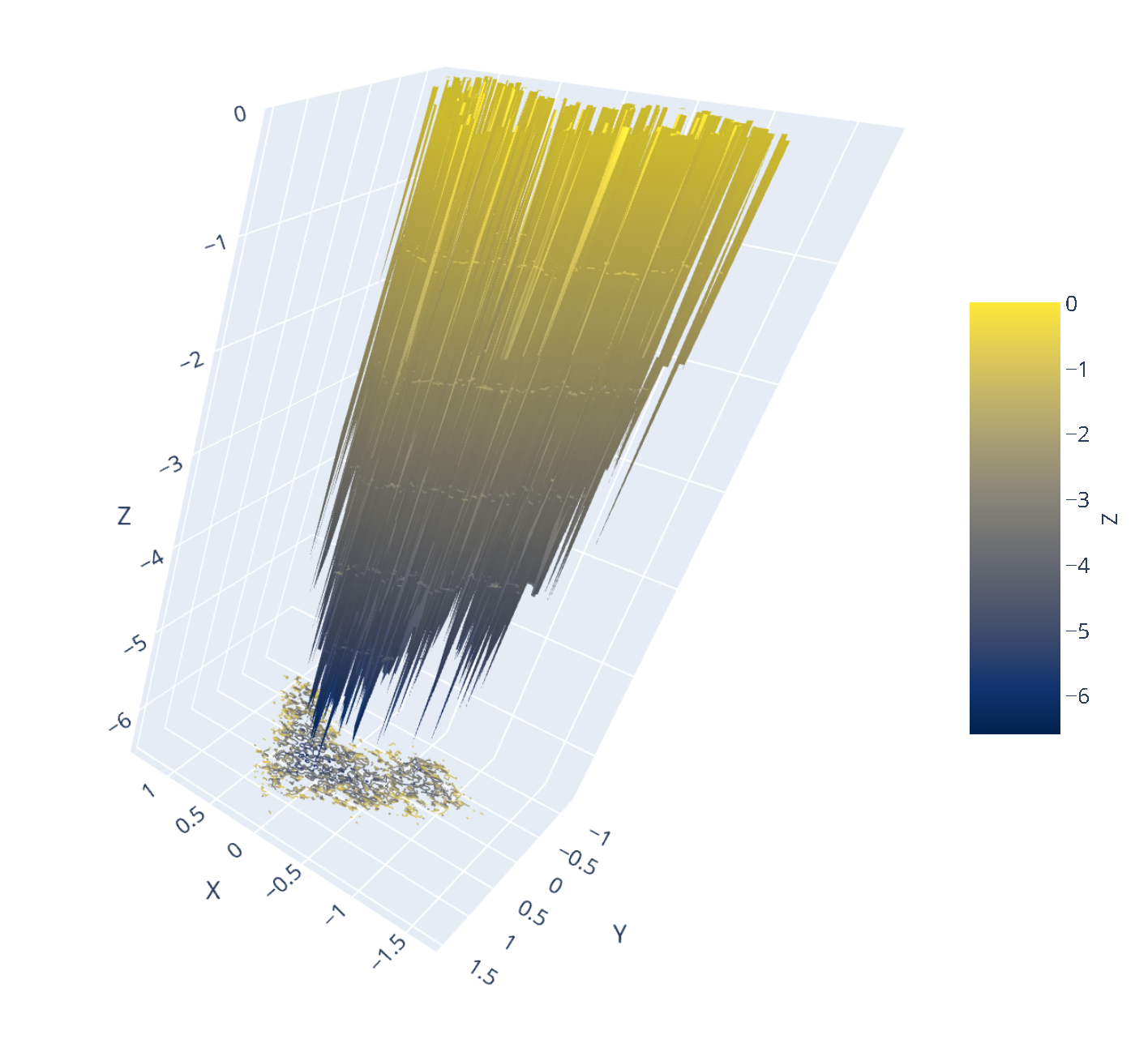
7.14. Interactive 3D FES Using md-davis

The construction of an interactive 3D plot of the FES from the data generated by GROMACS is powered by md-davis, a Python3 package and tool developed by Maity et al., 2022. The Rg-RMSD FES and the principal component-derived FES plots are shown below. Click on the image to view the interactive plots.

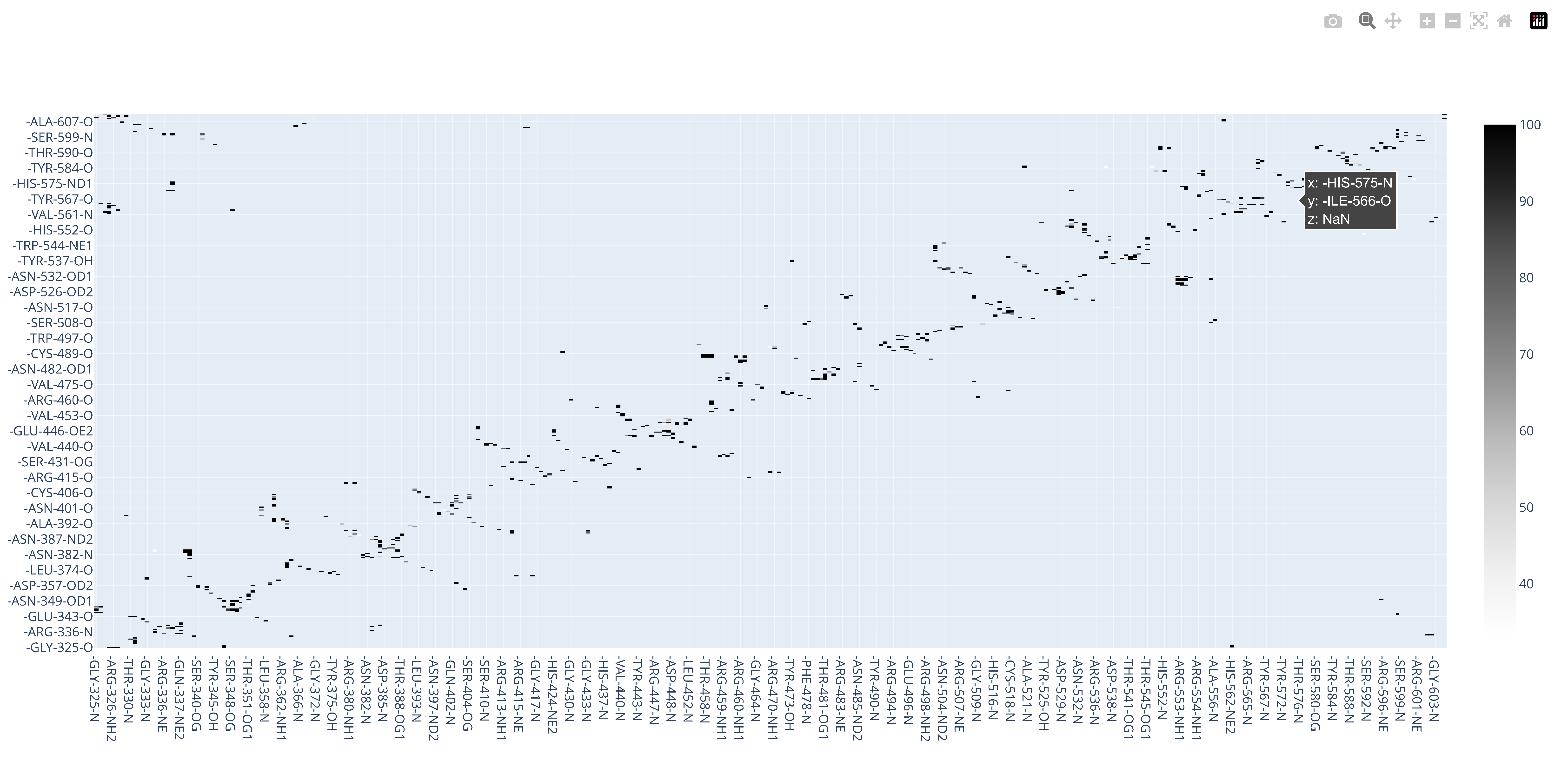
7.15. Interactive Hydrogen Bond Matrix Using md-davis

The hydrogen bond matrix is generated by md-davis, which uses the hydrogen bond data produced by GROMACS. You can check the details of how md-davis does this here and the details of how CHAPERONg implements it here. As shown below, md-davis produces an informative and interactive .html plot which can be opened in a browser. Click on the image to view the plot.

There are more in-depth analyses that we can do with the simulation data using CHAPERONg. You can find these out by further exploring the tool. In the next tutorial, we will run a longer simulation, save more coordinates, and carry out a more detailed analysis of the simulation trajectory.

I try my best to make the information on this website as accurate as possible, but if you find any errors in the contents of this page or any other page on this website, kindly get in touch with me at contact@abeebyekeen.com. Also, you are welcome to reach out for assistance and collaboration.